Tail Drop, Global Synchronization, and TCP Starvation

Congestion-Avoidance Concepts and Random Early Detection (RED) 433

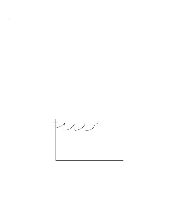
rate, with even more significant throughput improvements, because avoiding congestion and tail drops decreases the overall number of lost packets. Figure 6-4 shows an example graph of the same interface, after WRED was applied.

Figure 6-4 Graph of Traffic Rates After the Application of WRED

Line Rate

Actual Rate

with WRED

Average Rate

Before WRED

Another problem can occur if UDP traffic competes with TCP for bandwidth and queue space. Although UDP traffic consumes a much lower percentage of Internet bandwidth than TCP does, UDP can get a disproportionate amount of bandwidth as a result of TCP’s reaction to packet loss. Imagine that on the same Internet router, 20 percent of the offered packets were UDP, and 80 percent TCP. Tail drop causes some TCP and UDP packets to be dropped; however, because the TCP senders slow down, and the UDP senders do not, additional UDP streams from the UDP senders can consume more and more bandwidth during congestion.

Taking the same concept a little deeper, imagine that several people crank up some UDP-based audio or video streaming applications, and that traffic also happens to need to exit this same congested interface. The interface output queue on this Internet router could fill with UDP packets. If a few high-bandwidth UDP applications fill the queue, a larger percentage of TCP packets might get tail dropped—resulting in further reduction of TCP windows, and less TCP traffic relative to the amount of UDP traffic.

The term “TCP starvation” describes the phenomena of the output queue being filled with larger volumes of UDP, causing TCP connections to have packets tail dropped. Tail drop does not distinguish between packets in any way, including whether they are TCP or UDP, or whether the flow uses a lot of bandwidth or just a little bandwidth. TCP connections can be starved for bandwidth because the UDP flows behave poorly in terms of congestion control. Flow-Based WRED (FRED), which is also based on RED, specifically addresses the issues related to TCP starvation, as discussed later in the chapter.

434 Chapter 6: Congestion Avoidance Through Drop Policies

Random Early Detection (RED)

Random Early Detection (RED) reduces the congestion in queues by dropping packets so that some of the TCP connections temporarily send fewer packets into the network. Instead of waiting until a queue fills, causing a large number of tail drops, RED purposefully drops a percentage of packets before a queue fills. This action attempts to make the computers sending the traffic reduce the offered load that is sent into the network.

The name “Random Early Detection” itself describes the overall operation of the algorithm. RED randomly picks the packets that are dropped after the decision to drop some packets has been made. RED detects queue congestion early, before the queue actually fills, thereby avoiding tail drops and synchronization. In short, RED discards some randomly picked packets early, before congestion gets really bad and the queue fills.

RED logic contains two main parts. RED must first detect when congestion occurs; in other words, RED must choose under what conditions it should discard packets. When RED decides to discard packets, it must decide how many to discard.

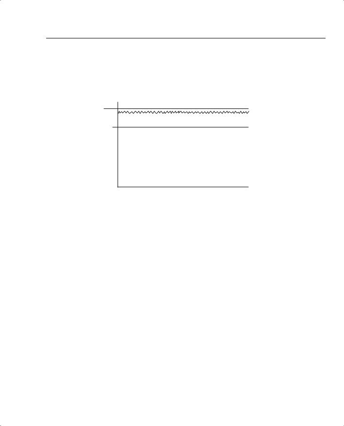
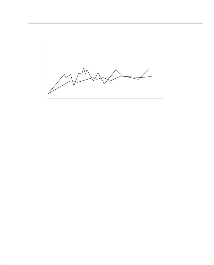
First, RED measures the average queue depth of the queue in question. RED calculates the average depth, and then decides whether congestion is occurring based on the average depth. RED uses the average depth, and not the actual queue depth, because the actual queue depth will most likely change much more quickly than the average depth. Because RED wants to avoid the effects of synchronization, it needs to act in a balanced fashion, not a jerky, sporadic fashion. Figure 6-5 shows a graph of the actual queue depth for a particular queue, compared with the average queue depth.

As seen in the graph, the calculated average queue depth changes more slowly than does the actual queue depth. RED uses the following algorithm when calculating the average queue depth:

New average = (Old_average * (1 – 2–n)) + (Current_Q_depth * 2–n)

For you test takers out there, do not worry about memorizing the formula, but focus on the idea. WRED uses this algorithm, with a default for n of 9. This makes the equation read as follows:

New average = (Old_average * .998) + (Current_Q_depth * .002)

Congestion-Avoidance Concepts and Random Early Detection (RED) 435

Figure 6-5 Graph of Actual Queue Depth Versus Average Queue Depth

In other words, the current queue depth only accounts for .2 percent of the new average each time it is calculated. Therefore, the average changes slowly, which helps RED prevent overreaction to changes in the queue depth. When configuring WRED and FRED, you can change the value of n in this formula by setting the exponential weighting constant parameter. By making the exponential weighting constant smaller, you make the average change more quickly; by making it larger, the average changes more slowly.

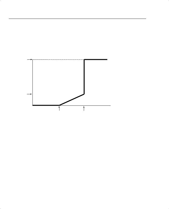
RED decides whether to discard packets by comparing the average queue depth to two thresholds, called the minimum threshold and maximum threshold. Table 6-2 describes the overall logic of when RED discards packets, as illustrated in Figure 6-6.

Table 6-2 Three Categories of When RED Will Discard Packets and How Many

As seen in Table 6-2 and Figure 6-6, RED does not discard packets when the average queue depth falls below the minimum threshold. When the average depth rises above the maximum threshold, RED discards all packets. In between the two thresholds, however, RED discards a percentage of packets, with the percentage growing linearly as the average queue depth grows. The core concept behind RED becomes more obvious if you notice that the maximum percentage of packets discarded is still much less than discarding all packets. Once again, RED wants

436 Chapter 6: Congestion Avoidance Through Drop Policies

to discard some packets, but not all packets. As congestion increases, RED discards a higher percentage of packets. Eventually, the congestion can increase to the point that RED discards all packets.

Figure 6-6 RED Discarding Logic Using Average Depth, Minimum Threshold, and Maximum Threshold

Discard

Percentage

100%

Maximum

Discard

Percentage

Average Queue Depth

Minimum Threshold Maximum Threshold

You can set the maximum percentage of packets discarded by WRED by setting the mark probability denominator (MPD) setting in IOS. IOS calculates the maximum percentage using the formula 1/MPD. For instance, an MPD of 10 yields a calculated value of 1/10, meaning the maximum discard rate is 10 percent.

Table 6-3 summarizes some of the key terms related to RED.