Queuing Tools 257

2Tail drop is the only available drop policy.

3Sixteen queues maximum.

4You can set the queue length to zero, which means the queue has theoretically infinite length. Default is 20 per queue.

5Inside a queue, CQ uses FIFO logic.

6When scheduling among the queues, CQ services the configured byte count per queue during a continuous round-robin through the queues.

CQ works great for networks with no jitter-sensitive applications that also need to reserve general percentages of link bandwidth for different classes of traffic. CQ does not provide lowlatency service, like PQ’s High queue does, although it does allow each queue to receive some service when the link is congested. Table 4-4 summarizes some of the key features of CQ. For those of you pursuing the QoS exam, look at Appendix B for details of how to configure CQ.

Weighted Fair Queuing (WFQ)

Weighted Fair Queuing differs from PQ and CQ in several significant ways. The first and most obvious difference is that WFQ does not allow classification options to be configured! WFQ classifies packets based on flows. A flow consists of all packets that have the same source and destination IP address, and the same source and destination port numbers. So, no explicit matching is configured. The other large difference between WFQ versus PQ and CQ is the scheduler, which simply favors low-volume, higher-precedence flows over large-volume, lower-precedence flows. Also because WFQ is flow based, and each flow uses a different queue,

258 Chapter 4: Congestion Management

the number of queues becomes rather large—up to a maximum of 4096 queues per interface. And although WFQ uses tail drop, it really uses a slightly modified tail-drop scheme—yet another difference.

IOS provides several variations of WFQ as well. This section concentrates on WFQ, whose longer, more descriptive name is Flow-Based WFQ. For those of you taking the QoS exam, Appendix B covers several variations of WFQ—namely, distributed WFQ (dWFQ), ToS-based dWFQ, and QoS group-based dWFQ. Each has slight variations to the baseline concepts and configuration of WFQ.

Ironically, WFQ requires the least configuration of all the queuing tools in this chapter, yet it requires the most explanation to achieve a deep understanding. The extra work to read through the details will certainly help on the exam, plus it will give you a better appreciation for WFQ, which may be the most pervasively deployed QoS tool in Cisco routers.

WFQ Classification

Flow-Based WFQ, or just WFQ, classifies traffic into flows. Flows are identified by at least five items in an IP packet:

•Source IP address

•Destination IP ADDRESS

•Transport layer protocol (TCP or UDP) as defined by the IP Protocol header field

•TCP or UDP source port

•TCP or UDP destination port

Depending on what document you read, WFQ also classifies based on the ToS byte. In particular, the CCIP QoS exam expects WFQ to classify based on the ToS byte as well as the five items listed previously. The DQOS course, and presumably the DQOS exam, claims that it classifies on the five fields listed previously. Most documentation just lists the five fields in the preceding list. (As with all items that may change with later releases of the exams and courses, look to www.ciscopress.com/1587200589 for the latest information.)

Whether WFQ uses the ToS byte or not when classifying packets, practically speaking, does not matter much. Good design suggests that packets in a single flow ought to have their Precedence or DSCP field set to the same value—so the same packets would get classified into the same flow, regardless of whether WFQ cares about the ToS byte or not for classification.

The term “flow” can have a couple of different meanings. For instance, imagine a PC that is downloading a web page. The user sees the page appear, reads the page for 10 seconds, and clicks a button. A second web page appears, the user reads the page for 10 seconds, and clicks

Queuing Tools 259

another button. All the pages and objects came from a single web server, and all the pages and objects were loaded using a single TCP connection between the PC and the server. How many different combinations of source/destination, address/port, and transport layer protocol, are used? How many different flows?

From a commonsense perspective, only one flow exists in this example, because only one TCP connection is used. From WFQ’s perspective, no flows may have occurred, or three flows existed, and possibly even more. To most people, a single TCP flow exists as long as the TCP connection stays up, because the packets in that connection always have the same source address, source port, destination address, and destination port information. However, WFQ considers a flow to exist only as long as packets from that flow are queued to be sent out of an interface. For instance, while the user is reading the web pages for 10 seconds, the routers finish sending all packets sent by the web server, so the queue for that flow is empty. Because the intermediate routers had no packets queued in the queue for that flow, WFQ removes the flow. Similarly, even while transferring different objects that comprise a web page, if WFQ empties a flow’s queue, it removes the queue, because it is no longer needed.

Why does it matter that flows come and go quickly from WFQ’s perspective? With class-based schemes, you always know how many queues you have, and you can see some basic statistics for each queue. With WFQ, the number of flows, and therefore the number of queues, changes very quickly. Although you can see statistics about active flows, you can bet on the information changing before you can type the show queue command again. The statistics show you information about the short-lived flow—for instance, when downloading the third web page in the previous example, the show queue command tells you about WFQ’s view of the flow, which began when the third web page was being transferred, not when the TCP connection was formed.

WFQ Scheduler: The Net Effect

Cisco publishes information about how the WFQ scheduler works. Even with an understanding of how the scheduler works, however, the true goals behind the scheduler are not obvious. This section reflects on what WFQ provides, and the following sections describe how WFQ accomplishes the task.

The WFQ scheduler has two main goals. The first is to provide fairness among the currently existing flows. To provide fairness, WFQ gives each flow an equal amount of bandwidth. If 10 flows exist for an interface, and the clock rate is 128 kbps, each flow effectively gets 12.8 kbps. If 100 flows exist, each flow gets 1.28 kbps. In some ways, this goal is similar to a time-division multiplexing (TDM) system, but the number of time slots is not preset, but instead based on the number of flows currently exiting an interface. Also keep in mind that the concept of equal shares of bandwidth for each flow is a goal—for example, the actual scheduler logic used to accomplish this goal is much different from the bandwidth reservation using byte counts with CQ.

260 Chapter 4: Congestion Management

With each flow receiving its fair share of the link bandwidth, the lower-volume flows prosper, and the higher-volume flows suffer. Think of that 128-kbps link again, for instance, with 10 flows. If Flow 1 needs 5 kbps, and WFQ allows 12.8 kbps per flow, the queue associated with Flow 1 may never have more than a few packets in it, because the packets will drain quickly. If Flow 2 needs 30 kbps, then packets will back up in Flow 2’s queue, because WFQ only gives this queue 12.8 kbps as well. These packets experience more delay and jitter, and possibly loss if the queue fills. Of course, if Flow 1 only needs 5 kbps, the actual WFQ scheduler allows other flows to use the extra bandwidth.

The second goal of the WFQ scheduler is to provide more bandwidth to flows with higher IP precedence values. The preference of higher-precedence flows is implied in the name—

“Weighted” implies that the fair share is weighted, and it is weighted based on precedence. With 10 flows on a 128-kbps link, for example, if 5 of the flows use precedence 0, and 5 use precedence 1, WFQ might want to give the precedence 1 flows twice as much bandwidth as the precedence 0 flows. Therefore, 5 precedence 0 flows would receive roughly 8.5 kbps each, and 5 precedence 1 flows would receive roughly 17 kbps each. In fact, WFQ provides a fair share roughly based on the ratio of each flow’s precedence, plus one. In other words, precedence 7 flows get 8 times more bandwidth than does precedence 0 flows, because (7 + 1) / (0 + 1) = 8. If you compare precedence 3 to precedence 0, the ratio is roughly (3 + 1) / (0 + 1) = 4.

So, what does WFQ accomplish? Ignoring precedence for a moment, the short answer is lowervolume flows get relatively better service, and higher-volume flows get worse service. Higherprecedence flows get better service than lower-precedence flows. If lower-volume flows are given higher-precedence values, the bandwidth/delay/jitter/loss characteristics improve even more. In a network where most of the delay-sensitive traffic is lower-volume traffic, WFQ is a great solution. It takes one command to enable it, and it is already enabled by default! Its default behavior favors lower-volume flows, which may be the more important flows. In fact, WFQ came out when many networks’ most important interactive flows were Telnet and Systems Network Architecture (SNA) encapsulated in IP. These types of flows used much less volume than other flows, so WFQ provided a great default, without having to worry about how to perform prioritization on encapsulated SNA traffic.

WFQ Scheduling: The Process

WFQ gives each flow a weighted percentage of link bandwidth. However, WFQ does not predefine queues like class-based queuing tools do, because WFQ dynamically classifies queues based on the flow details. And although WFQ ends up causing each flow to get some percentage of link bandwidth, the percentage changes, and changes rapidly, because flows come and go frequently. Because each flow may have different precedence values, the percentage of link bandwidth for each flow will change, and it will change very quickly, as each flow is added or removed. In short, WFQ simply could not be implemented by assigning a percentage of bandwidth, or a byte count, to each queue.

Queuing Tools 261

The WFQ scheduler is actually very simple. When the TX Queue/Ring frees a slot, WFQ can move one packet to the TX Queue/Ring, just like any other queuing tool. The WFQ scheduler takes the packet with the lowest sequence number (SN) among all the queues, and moves it to the TX Queue/Ring. The SN is assigned when the packet is placed into a queue, which is where the interesting part of WFQ scheduling takes place.

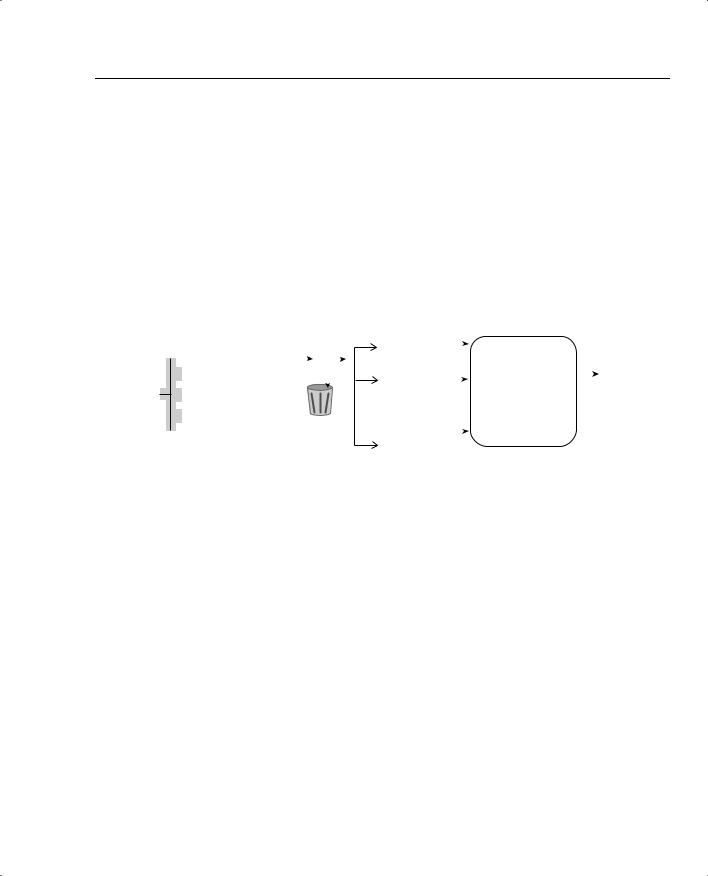
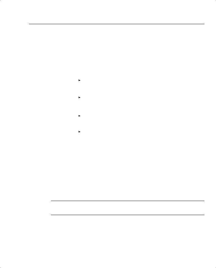
For perspective on the sequence of events, marking the SN, and serving the queues, examine Figure 4-13.

Figure 4-13 WFQ: Assigning Sequence Numbers and Servicing Queues

3)Maximum Number of Queues

4)Maximum Queue Length

WFQ calculates the SN before adding a packet to its associated queue. In fact, WFQ calculates the SN before making the drop decision, because the SN is part of the modified tail-drop logic. The WFQ scheduler considers both packet length and precedence when calculating the SN. The formula for calculating the SN for a packet is as follows:

Previous_SN + weight * new_packet_length

The formula considers the length of the new packet, the weight of the flow, and the previous SN. By considering the packet length, the SN calculation results in a higher number for larger packets, and a lower number for smaller packets. The formula considers the SN of the most recently enqueued packet in the queue for the new sequence number. By including the SN of the previous packet enqueued into that queue, the formula assigns a larger number for packets in queues that already have a larger number of packets enqueued.

The third component of the formula, the weight, is the most interesting part. We know from the basic scheduling algorithm that the lowest SN is taken next, and we know that WFQ wants to give more bandwidth to the higher-precedence flows. So, the weight values are inversely proportional to the precedence values. Table 4-5 lists the weight values used by WFQ before and after the release of 12.0(5)T/12.1.

262 Chapter 4: Congestion Management

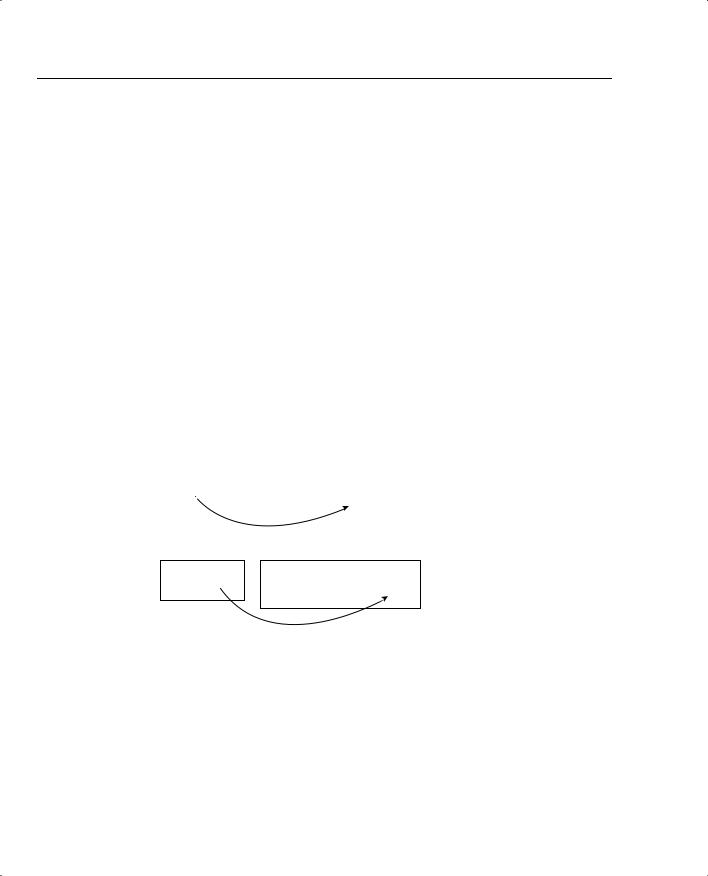
As seen in the table, the larger the precedence value, the lower the weight making the SN lower. An example certainly helps for a fuller understanding. Consider the example in Figure 4-14, which illustrates one existing flow and one new flow.

Figure 4-14 WFQ Sequence Number Assignment Example

New Flow: Flow 2

New packet 2, Flow 2:

Length 500,

Precedence 0

SN = 100 + 32384*500 = 16,192,100

When adding new packet 1 to the queue for Flow 1, WFQ just runs the formula against the length of the new packet (100) and the weight, adding the SN of the last packet in the queue to which the new packet will be added. For new flows, the same formula is used; because there are no other packets in the queue, however, the SN of the most recently sent packet, in this case 100, is used in the formula. In either case, WFQ assigns larger SN values for larger packets and for those with lower IP precedence.

Queuing Tools 263

A more detailed example can show some of the effects of the WFQ SN assignment algorithm and how it achieves its basic goals. Figure 4-15 shows a set of four flow queues, each with four packets of varying lengths. For the sake of discussion, assume that the SN of the previously sent packet is zero in this case. Each flow’s first packet arrives at the same instant in time, and all packets for all flows arrive before any more packets can be taken from the WFQ queues.

Figure 4-15 WFQ Sequence Number Assignment Example 2

In this example, each flow had four packets arrive, all with a precedence of zero. The packets in Flow 1 were all 1500 bytes in length; in Flow 2, the packets were 1000 bytes in length; in Flow 3, they were 500 bytes; and finally, in Flow 4, they were 100 bytes. With equal precedence values, the Flow 4 packets should get better service, because the packets are much smaller. In fact, all four of Flow 1’s packets would be serviced before any of the packets in the other flows. Flow 3’s packets are sent before most of the packets in Flow 1 and Flow 2. Thus, the goal of giving the lower-volume flows better service is accomplished, assuming the precedence values are equal.

NOTE For the record, the order the packets would exit the interface, assuming no other events occur, is 13 first, then 14, followed by 15, 16, 9, 5, 19, 1, 11, 6, 12, 2, 7, 8, 3, 4.

To see the effect of different precedence values, look at Figure 4-16, which lists the same basic scenario but with varying precedence values.