


184 • Chapter 5 • Competitors and Competition
firms’ reaction functions simultaneously. In our present example, this solution is Q* 5
1
Q* 5 30. Graphically, this corresponds to the point in Figure 5.2 where the two reac-
2
tion functions intersect. We can also solve for the equilibrium market price P* and the profits each firm earns. Recalling that P 5 100 2 Q1 2 Q2, we find that P* 5 $40. Substituting price and quantity into the equation for each firm’s profits reveals that each firm makes $900 in profit in equilibrium.
Cournot’s assumption that firms will simultaneously select the best response to each other’s choices seems rather demanding. How are firms supposed to make such accurate guesses about each other’s output? Yet as a focal point for analysis, this assumption may not be too bad. It means that in equilibrium, each firm will be happy with its choice of output, which seems more satisfying than assuming that each firm is consistently unhappy with its choice. Moreover, neither Hynix nor Micron need be omniscient for the Cournot equilibrium quantities to emerge. Suppose that both firms are “out of equilibrium” in the sense that at least one firm has chosen to produce a quantity other than 30. For example, suppose that Q1 5 Q2 5 40. Neither firm will be happy with its choice of quantity—each is producing more than it would like given its rival’s production. As a result, we would expect each firm to adjust to the other firm’s choices.
Table 5.5 shows an example of the adjustment process. Suppose that Hynix makes the first adjustment. It examines its profit-maximization equation and determines that if Q2 5 40, it should choose Q1 5 25. Suppose now that Hynix reduces its output to 25. Micron will examine its own profit-maximization equation and determine that if Hynix chooses Q1 5 25, then it should choose Q2 5 32.5. Table 5.5 shows that Q1 and Q2 continue to converge toward the equilibrium values of Q1 5 Q2 5 30.
The Revenue Destruction Effect
In the Cournot model, equilibrium industry output does not maximize industry profit. Industry profit is maximized at the monopoly quantity and price computed earlier—45 units of output sold at $55 each. By independently maximizing their own profits, firms produce more output than they would if they collusively maximized industry profits. This is characteristic of oligopolistic industries: The pursuit of individual self-interest does not maximize the profits of the group as a whole. This occurs under Cournot competition for the following reason. When one firm, say Hynix, expands its output, it reduces the market price. This reduces revenues from all customers who would have purchased DRAM chips at the higher price. This is known as the revenue destruction effect. Unlike a monopolist, which would bear the full burden of the revenue destruction effect, Hynix shares this burden with Micron. Thus, Hynix expands its production volume more aggressively than it would if it were a monopolist,
TABLE 5.5
The Cournot Adjustment Process
Starting Q1 |
Starting Q2 |
Firm That Is Adjusting |
Ending Q1 |
Ending Q2 |
40 |
40 |
Firm 1 |
25 |
40 |
25 |
40 |
Firm 2 |
25 |
32.5 |
25 |
32.5 |
Firm 1 |
28.75 |
32.5 |
28.75 |
32.5 |
Firm 2 |
28.75 |
30.63 |
28.75 |
30.63 |
Firm 1 |
29.69 |
30.63 |
|
|
|
|
|
Oligopoly • 185
TABLE 5.6
Cournot Equilibria as the Number of Firms Increases
Number of Firms |
Market Price |
Market Quantity |
Per-Firm Profits |
Total Profits |
2 |
$40 |
60 |
$900 |
$1,800 |
3 |
$32.5 |
67.5 |
$506.25 |
$1,518.75 |
5 |
$25 |
75 |
$225 |
$1,125 |
10 |
$18.2 |
81.8 |
$66.94 |
$669.40 |
100 |
$10.9 |
89.1 |
$0.79 |
$79 |
|
|
|
|
|
or if it was trying to maximize industry profit. Micron will do likewise, driving the oligopoly price well below the monopoly price.
The revenue destruction effect helps explain why small firms are often most willing to disrupt pricing stability. Firms of all sizes enjoy the same benefit when they expand output by a given amount, but smaller firms suffer a smaller revenue destruction effect, which is instead borne mainly by their larger rivals. The revenue destruction effect also explains why the Cournot equilibrium price falls as the number of firms in the market increases. Each firm has, on average, a smaller share of the market and so bears a smaller share of the revenue destruction effect. Table 5.6 illustrates this point by showing equilibrium prices, profits, and outputs in a Cournot industry with the same demand curve and cost function as in the preceding example. The equilibrium price and profit per firm decline as the number of firms increases. More generally, it can be shown that the average PCM of a firm in a Cournot equilibrium is given by the formula PCM 5 H/ , where H denotes the Herfindahl and is the price elasticity of market demand. Thus, the less concentrated the industry (the lower the industry’s H), the smaller will be PCMs in equilibrium.
Cournot’s Model in Practice
Antitrust enforcers often use the Herfindahl index to predict the effects of a merger on pricing. Cournot’s model provides a justification for this approach; in markets where firms behave as Cournot describes, one can compute how a merger will affect the Herfindahl index and use the results of the Cournot model to predict the change in price. Because many factors besides market concentration may ultimately affect equilibrium output and price, computation of the Herfindahl is usually just the first step in merger analysis. We will discuss additional factors in the next two chapters.
The Cournot model has another practical use. It is very straightforward to alter one or more parameters of the model—the demand curve and firm costs—and recompute equilibria. This makes it possible to forecast how changes in demand and costs will affect profitability in markets in which firms behave according to the Cournot equilibrium assumption. This makes the Cournot model a valuable tool for planning.
Bertrand Price Competition
In Cournot’s model, each firm selects a quantity to produce, and the resulting total output determines the market price. Alternatively, one might imagine a market in which each firm selects a price and stands ready to meet all the demand for its product at that price. This model of competition was first analyzed by Joseph Bertrand

186 • Chapter 5 • Competitors and Competition
EXAMPLE 5.5 COURNOT EQUILIBRIUM IN THE CORN WET MILLING INDUSTRY
Michael Porter and Michael Spence’s case study of the corn wet milling industry is a realworld illustration of the Cournot model.16 Firms in the corn wet milling industry convert corn into cornstarch and corn syrup. The corn syrup industry was a fairly stable oligopoly until the 1960s, when several firms entered the market, including Archer-Daniels-Midland and Cargill. The new competitors and new capacity disrupted the old equilibrium and drove prices downward. By the early 1970s, however, competitive stability returned to the industry as capacity utilization rates and prices rose. In 1972, a major development hit the industry: the production of high-fructose corn syrup (HFCS) became commercially viable. HFCS can be used instead of sugar to sweeten products, such as soft drinks. With sugar prices expected to rise, a significant market for HFCS beckoned. Firms in the corn wet milling industry had to decide whether and how to add capacity to accommodate the expected demand.
Porter and Spence studied this capacity expansion process. They did so through a detailed simulation of competitive behavior based on an in-depth study of the 11 major competitors in the industry. Porter and Spence postulated that each firm’s expansion decision was based on a conjecture about the overall expansion of industry capacity, as well as expectations about demand and sugar prices. Their model also took into account that capacity choices coupled with demand conditions determined industry prices of cornstarch, corn syrup, and HFCS. The notion that a firm’s capacity choice is based on conjectures about the capacity choices of other firms is directly analogous to the idea in the Cournot model that each firm bases its output choice on conjectures of the output choices of other firms. The notion that capacity decisions then deter-
mine a market price is also analogous to the Cournot model.
Porter and Spence’s simulation of the industry attempted to find an “equilibrium”: an industry capacity expansion path that, when each firm made its optimal capacity decision based on the conjecture that this path would prevail, resulted in an actual pattern of capacity expansion that matched the assumed pattern. This is directly analogous to the notion of a Cournot equilibrium, in which each firm’s expectations about the behavior of its competitors are confirmed by their actual behavior. Based on their simulation of industry decision making, Porter and Spence determined that an industry equilibrium would result in a moderate amount of additional capacity added to the industry as a result of the commercialization of HFCS. The specific predictions of their model compared with the actual pattern of capacity expansion are shown below.
Though not perfect, Porter and Spence’s calculated equilibrium comes quite close to the actual pattern of capacity expansion in the industry, particularly in 1973 and 1974. The discrepancies in 1975 and 1976 mainly reflect timing. Porter and Spence’s equilibrium model did not consider capacity additions in the years beyond 1976. In 1976, however, the industry had more than 4 billion pounds of HFCS capacity under construction, and that capacity did not come on line until after 1976. Including this capacity, the total HFCS capacity expansion was 9.2 billion pounds, as compared with the 9.1 billion pounds of predicted equilibrium capacity. Porter and Spence’s research suggests that a Cournot-like model, when adapted to the specific conditions of the corn wet milling industry, provided predictions that came remarkably close to the actual pattern of capacity expansion decisions.
|
|
Post-1973 |
1974 |
1975 |
1976 |
1976 |
Total |
|
|
Actual industry capacity |
0.6 |
1.0 |
1.4 |
2.2 |
4 |
9.2 (billions of lb) |
|
|
Predicted equilibrium capacity |
0.6 |
1.5 |
3.5 |
3.5 |
0 |
9.1 |
|
|
|
|
|
|
|
|
|
|
|
|
|
|
|
|
|
|
|
Oligopoly • 187
in 1883.17 In Bertrand’s model, each firm selects a price to maximize its own profits, given the price that it believes the other firm will select. Each firm also believes that its pricing practices will not affect the pricing of its rival; each firm views its rival’s price as fixed.
We can use the cost and demand conditions from the Cournot model to explore the Bertrand market equilibrium, again using the (hypothetical) example of rival DRAM producers Hynix and Micron. (Recall that firm 1 is Hynix and firm 2 is Micron.) We saw earlier that when MC1 5 MC2 5 $10, and demand is given by P 5 100 2 Q1 2 Q2, the Cournot equilibrium is Q1 5 Q2 5 30 and P1 5 P2 5 $40. This is not, however, a Bertrand equilibrium, because each firm believes it can capture the entire market by slightly undercutting its rival’s price. For example, if P2 5 $40 and P1 5 $39, then Q1 5 61 and Q2 5 0. As a result, Hynix earns profits of $1,769, well above the profits of $900 it would earn if it matched Micron’s price of $40.
Of course, P1 5 $39 and P2 5 $40 cannot be an equilibrium either because at these prices, Micron will want to undercut Hynix’s price. As long as both firms set prices that exceed marginal costs, one firm will always have an incentive to slightly undercut its competitor. This implies that the only possible equilibrium is P1 5 P2 5 marginal cost 5 $10. At these prices, neither firm can do better by changing its price. If either firm lowers price, it will lose money on each unit sold. If either firm raises price, it would sell nothing.
In Bertrand’s model with firms producing identical products, rivalry between two firms results in the perfectly competitive outcome. When firms’ products are differentiated, as in monopolistic competition, price competition is less intense. (Later in this chapter, we will examine Bertrand price competition when firms produce differentiated products.) Bertrand competition can destabilize markets where firms must incur sunk costs to do business, because there is not enough variable profit to cover the sunk costs. If one firm should exit the market, the remaining firm could try to raise its price. But this might simply attract a new entrant that will wrest away some of the remaining firm’s business. Price competition may be limited if one or both firms runs up against a capacity constraint and cannot readily steal market share, or if the firms learn to stop competing on the basis of price. These ideas are covered in greater depth in Chapter 7.
Why Are Cournot and Bertrand Different?
The Cournot and Bertrand models make dramatically different predictions about the quantities, prices, and profits that will arise under oligopolistic competition. One way to reconcile the two models is to recognize that Cournot and Bertrand competition may take place over different time frames. Cournot competitors can be thought of as choosing capacities and then competing as capacity-constrained price setters. The result of this “two-stage” competition (first choose capacities and then choose prices) is identical to the Cournot equilibrium in quantities.18 More cutthroat Bertrand competition results if the competitors are no longer constrained by their capacity choices, either because demand declines or a competitor miscalculates and adds too much capacity.
Another way to reconcile the models is to recognize that they make different assumptions about how firms expect their rivals to react to their own competitive moves. The Cournot model applies most naturally to markets in which firms must make production decisions in advance, are committed to selling all of their output, and are therefore unlikely to react to fluctuations in the rivals’ output. This might occur if the majority of production costs are sunk, or because it is costly to hold

188 • Chapter 5 • Competitors and Competition
EXAMPLE 5.6 COMPETITION AMONG U.S. HEALTH INSURERS
Few businesses are as reviled as health insurance. Insurers sell an intangible product (protection against financial risk), they seem to avoid selling to customers who need their product the most, and administrative snafus seem to take place at the worst possible time for patients. Critics complain that insurers make money off the backs of sick people, though the reality is that insurers make money when their customers stay healthy. Despite public perceptions, health insurers have often struggled to make a profit, though several have posted record profits in recent years. These public perceptions and management challenges all reflect a unique history and competitive environment.
The first insurance companies emerged during the Great Depression, when hospitals banded together and accepted annual upfront payments in exchange for guarantees of free care. These insurance arrangements came to be known as Blue Cross plans; Blue Shield plans for physicians followed shortly thereafter. The “Blues” were organized as nonprofit companies, enjoying tax breaks while promising not to exclude enrollees on the basis of prior illnesses. The Blues formed a trade association and agreed not to compete across geographic territories. Commercial (for-profit) insurers emerged during the 1950s, and the industry was soon split fairly evenly between the Blues and the Commercials. Aside from the Blues, there were few plans with substantial market shares, as entry was easy and most markets had many competitors.
Employer groups were (and remain) the largest purchasers of insurance. Insurers preferred selling to employer groups because they represented predictable risk pools. Aside from some of the rules governing the Blues, there was little differentiation among insurers. All insurers covered nearly all medical services,
reimbursed nearly all medical costs, and did not restrict a patient’s choice of provider. Employers mostly looked for insurers that offered low premiums and paid their bills promptly and accurately, although some national employers looked for national insurers such as Aetna and Prudential to simplify plan administration. As a result, insurers competed aggressively on price, and profit margins were thin.
The 1980s saw the emergence of health maintenance organizations (HMOs) and other forms of managed care. HMOs relied on innovative financial incentives and controversial restrictions on access to reduce medical spending. At first, there were only a handful of HMOs in each market; often the local Blue plan offered the only HMO. This gave the HMO an opportunity to prosper by setting premiums just below indemnity carriers, a practice known in the industry as “shadow pricing.” As managed care proliferated, plans tried to differentiate themselves on the basis of their provider networks, utilization controls, and service coverage. But these strategies were easily imitated, and by the mid-1990s, plans believed that the only way to thrive was to enroll as many customers as possible and try to leverage size into a sustainable advantage.
The resulting price war took its toll, and many HMOs lost money. At the same time, a backlash against the worst industry practices caused managed care plans to ease up on cost controls. As a result, many commercial plans have consolidated while several Blues plans have converted to for-profit status. Today, there are many metropolitan areas in which two or three carriers control nearly the entire market. Premiums are rising faster than the rate at which costs are rising, profits and executive compensation are at record highs, and a new backlash has begun.
inventories—commodities such as natural gas and copper come to mind. In such settings, firms will do what it takes to sell their output and will also believe that its competitors will keep to their planned sales levels. Thus, if a firm lowers its price, it cannot expect to steal customers from its rivals. Because “business stealing” is not an option,
Oligopoly • 189
Cournot competitors must share in the revenue destruction effect if they expand output. As a result, they set prices less aggressively than Bertrand competitors. Thus, the Cournot equilibrium outcome, while not the monopoly one, nevertheless results in positive profits and a price that exceeds marginal and average cost.
The Bertrand model pertains to markets in which capacity is sufficiently flexible that firms can meet all of the demand that arises at the prices they announce. If firms’ products are perfect substitutes, then each Bertrand competitor believes that it can steal massive amounts of business from its competitors through a small cut in price, effectively bearing none of the revenue destruction effect. In equilibrium, price–cost margins are driven to zero.
These distinctions help to explain the pro-cyclicality of airline industry profits. During business downturns, the airlines have substantial excess capacity on many routes. Because many consumers perceive the airlines as selling undifferentiated products, each airline can fill empty seats by undercutting rivals’ prices and stealing their customers. The resulting competition resembles Bertrand’s model and has led to substantial losses. During boom times, airlines operate near capacity and have little incentive to cut prices. Because they have few empty seats, they are unable to steal business even if they wanted to. Competition resembles Cournot’s model and allows the airlines to be profitable. In recent years, domestic U.S. airlines have withdrawn capacity by flying fewer flights and downsizing planes; this has helped stabilize pricing during downturns.
Many other issues may be considered when assessing the likely conduct and performance of firms in an oligopoly. Competition may be based on a variety of product parameters, including quality, availability, and advertising. Firms may not know the strategic choices of their competitors. The timing of decision making can profoundly influence profits. We discuss all of these issues in Chapter 7.
Bertrand Price Competition When Products
Are Horizontally Differentiated
In many oligopolistic markets, products are close, but not perfect, substitutes. The Bertrand model of price competition does not fully capture the nature of price competition in these settings. Fortunately, we can adapt the logic of the Bertrand model to deal with horizontally differentiated products.
When products are horizontally differentiated, a firm that lowers its price will only steal some if its rival’s customers. This discourages the kind of price cutting that takes place in the Bertrand model with identical products. To illustrate, consider the U.S. cola market. Farid Gasini, J. J. Lafont, and Quang Vuong (GLV) have used statistical methods to estimate demand curves for Coke (denoted by 1) and Pepsi (denoted by 2):19
Q1 5 63.42 2 3.98P1 1 2.25P2
Q2 5 49.52 2 5.48P2 1 1.40P1
With these demand functions, as Coke lowers its price below that of Pepsi, Coke’s demand rises gradually.
We can use the logic of the Cournot model to determine the price we expect each cola maker to charge. Because firms are choosing prices rather than quantities, this is called a differentiated Bertrand model. To solve for the differentiated Bertrand equilibrium, we will need information about demand (given above) as well as information
190 • Chapter 5 • Competitors and Competition
about marginal costs. GLV estimated that Coca-Cola had a constant marginal cost equal to $4.96, and Pepsi had a constant marginal cost of $3.96.
Armed with demand and cost data, we follow the same logic that we used to compute the Cournot equilibrium. We start by computing each firm’s profit-maximizing price as a function of its guess about its rival’s price. Coca-Cola’s profit can be written as its price–cost margin times the quantity it sells, which is given by its demand function.
ß1 5 (P1 2 4.96)(63.49 2 3.98P1 1 2.25P2g)
(We again use the subscript g to emphasize that Coca-Cola is making a guess about Pepsi’s price.) Using calculus to solve this maximization problem yields a reaction function20
P1 5 10.44 1 .2826P2g
Pepsi’s optimal price is derived similarly. It maximizes
ß2 5 (P2 2 3.94)(49.52 2 5.48P2 1 1.40P1g)
which yields a reaction function
P2 5 6.49 1 .1277P1g
As with the Cournot model, Coke and Pepsi could have reached conclusions like these using spreadsheet analysis. Despite what appears to be excessive mathematical formality, there is nothing unrealistic about this approach to modeling pricing decisions.
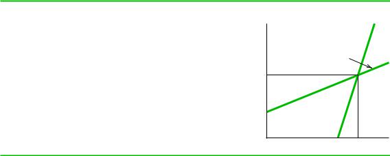
These reaction functions, displayed in Figure 5.3, are upward sloping.Thus, the lower the price the firm expects its rival to charge, the lower the price it should charge. In this sense, “aggressive” behavior by one firm (price cutting) is met by “aggressive” behavior by rivals. Note the contrast with the Cournot model, where “aggressive” behavior by one firm (output expansion) was met by “passive” behavior by rivals (output reduction).
Solving the two reaction functions simultaneously yields the Bertrand equilibrium in prices:
P1 5 $12.72
P2 5 $8.11
FIGURE 5.3
Bertrand Equilibrium with Horizontally Differentiated Products
Firm 1’s reaction function shows its profit-maximizing price for any price charged by firm 2. Firm 2’s reaction function shows its profit-maximizing price for any price charged by firm 1. The Bertrand equilibrium prices occur at the intersection of these reaction functions. In this example, this is at P1 5 $12.72 and P2 5 $8.11. At this point, each firm is choosing a profit-maximizing price, given the price charged by the other firm.
P2 |
|
Firm 1’s reaction |
|
function |
|
Firm 2’s reaction |
|
function |
|
$8.11 |
|
$6.49 |
|
$10.44 $12.72 |
P1 |