

Scale Economies, Indivisibilities, and the Spreading of Fixed Costs • 65
for total annual production of 125 million cans, then average fixed costs equal four cents per can. The underutilized plant is operating at a three-cent cost differential per can. In a price-competitive industry like aluminum can manufacturing, such a cost differential could make the difference between profit and loss.
Economies of Scale Due to Trade-offs among Alternative Technologies
Suppose that a firm is considering entering the can manufacturing business but does not anticipate being able to sell more than 125 million cans annually. Is it doomed to a three-cent-per-can cost disadvantage? The answer depends on the nature of the alternative production technologies and the planned production output. The fully automated technology described previously may yield the greatest cost savings when used to capacity, but it may not be the best choice at lower production levels. There may be an alternative that requires less initial investment, albeit with a greater reliance on ongoing expenses.
Suppose that the fixed costs of setting up a partially automated plant are $12.5 million, annualized to $1.25 million per year. The shortcoming of this plant is that it requires labor costs of one cent per can that are not needed at the fully automated plant. The cost comparison between the two plants is shown in Table 2.1.
Table 2.1 shows that while the fully automated technology has lower average total costs at high production levels, it is more costly at lower production levels. This is seen in Figure 2.3, which depicts average cost curves for both the fully and partially automated technologies. The curve labeled SAC1 is the average cost curve for a plant that has adopted the fully automated technology; the curve labeled SAC2 is the average cost curve for a plant that has adopted the partially automated technology. At output levels above 375 million, the fully automated technology has lower average total costs. At lower output levels, the partially automated technology is cheaper.
The aluminum can example demonstrates the difference between economies of scale that arise from increased capacity utilization with a given production technology and economies of scale that arise as a firm chooses among alternative production technologies. Reductions in average costs due to increases in capacity utilization are short-run economies of scale in that they occur within a plant of a given size. Reductions due to adoption of a technology that has high fixed costs but lower variable costs are long-run economies of scale. Given time to build a plant from scratch, a firm can
TABLE 2.1
Costs of Producing Aluminum Cans
500 Million Cans per Year |
125 Million Cans per Year |
Fully automated |
Average fixed costs 5 .01 |
|
Average labor costs 5 .00 |
|
Average materials costs 5 .03 |
|
Average total costs 5 .04 |
Partially automated |
Averge fixed costs 5 .0025 |
|
Averge labor costs 5 .01 |
|
Averge materials costs 5 .03 |
|
Averge total costs 5 .0425 |
Average fixed costs 5 .04 Average labor costs 5 .00 Average materials costs 5 .03 Average total costs 5 .07
Average fixed costs 5 .01 Average labor costs 5 .01 Average materials costs 5 .03 Average total costs 5 .05
66 • Chapter 2 • The Horizontal Boundaries of the Firm
FIGURE 2.3
Average Cost Curves for Can Production
SAC1 represents a high fixed/low variable cost technology. SAC2 represents a low fixed cost/high variable cost technology. At low levels of output, it is cheaper to use the latter technology. At high outputs, it is cheaper to use the former.
$ Per can
SAC2
SAC1
375
Millions of cans per year
choose the plant that best meets its production needs, avoiding excessive fixed costs if production is expected to be low, and excessive capacity costs if production is expected to be high.
Figure 2.4 illustrates the distinction between short-run and long-run economies of scale. (The Economics Primer discusses this distinction at length.) SAC1 and SAC2, which duplicate the cost curves in Figure 2.3, are the short-run average cost curves for the partially automated and fully automated plants, respectively. If we trace out the lower regions of each curve, we see the long-run average cost curve. The long-run average cost curve is everywhere on or below each short-run average cost curve. This reflects the flexibility that firms have to adopt the technology that is most appropriate for their forecasted output.
Regardless of plant size, firms that plan on exploiting scale economies must achieve the necessary throughput. Recall from Chapter 1 that throughput describes
FIGURE 2.4
Short-Run versus Long-Run Average Cost
In the long run, firms may choose their production technology as well as their output. Firms planning to produce beyond point X will choose the technology represented by SAC1. Firms planning to produce less than point X will choose the technology represented by SAC2. The heavy “lower envelope” of the two cost curves, which represents the lowest possible cost for each level of production, is called the long-run average cost curve.
$ Per can
X
SAC2
SAC1
375
Millions of cans per year

Scale Economies, Indivisibilities, and the Spreading of Fixed Costs • 67
EXAMPLE 2.1 HUB-AND-SPOKE NETWORKS AND ECONOMIES
OF SCOPE IN THE AIRLINE INDUSTRY
An important example of multiplant economies of scope arises in a number of industries in which goods and services are routed to and from several markets. In these industries, which include airlines, railroads, and telecommunications, distribution is organized around “hub- and-spoke” networks. In an airline hub-and- spoke network, an airline flies passengers from a set of “spoke” cities through a central “hub,” where passengers then change planes and fly from the hub to their outbound destinations. Thus, a passenger flying from, say, Omaha to Boston on United Airlines would board a United flight from Omaha to Chicago, change planes, and then fly from Chicago to Boston.
Recall that economies of scope occur when a firm producing many products has a lower average cost than a firm producing just a few products. In the airline industry, it makes economic sense to think about individual origin– destination pairs (e.g., Omaha to Boston, Chicago to Boston) as distinct products. Viewed in this way, economies of scope exist if an airline’s average cost is lower the more origin– destination pairs it serves. To understand how hub-and-spoke networks give rise to economies of scope, it is first necessary to explain economies of density. Economies of density are essentially economies of scale along a given route, that is, reductions in average cost as traffic volume on the route increases. (In the airline industry, traffic volume is measured as revenue-passenger miles [RPM], which is the number of passengers on the route multiplied by the number of miles, and average cost is the cost per revenue passenger mile.) Economies of density occur because of spreading flight-specific fixed costs (e.g., costs of the flight and cabin crew, fuel, aircraft servicing) and because of the economies of aircraft size. In the airline industry, trafficsensitive costs (e.g., food, ticket handling) are small in relation to flight-specific fixed costs. Thus, as its traffic volume increases, an airline can fill a larger fraction of its seats on a given type of aircraft (in airline industry lingo, it
increases its load factor—the ratio of passengers to available seats), and because the airline’s total costs increase only slightly, its cost per RPM falls as it spreads the flight-specific fixed costs over more traffic volume. As traffic volume on the route gets even larger, it becomes worthwhile to substitute larger aircraft (e.g., 300-seat Boeing 767s) for smaller aircraft (e.g., 150-seat Boeing 737s). A key aspect of this substitution is that the 300-seat aircraft flown a given distance at a given load factor is less than twice as costly as the 150-seat aircraft flown the same distance at the same load factor. The reason for this is that doubling the number of seats and passengers on a plane does not require doubling the sizes of flight and cabin crews or the amount of fuel used, and that the 300-seat aircraft is less than twice as costly to build as the 150-seat aircraft, owing to the cube-square rule, which will be discussed below.
Economies of scope emerge from the interplay of economies of density and the properties of a hub-and-spoke network. To see how, consider an origin–destination pair such as Omaha to Boston. This pair has a modest amount of daily traffic. An airline serving only this route would use small planes and operate with a relatively low load factor. But now consider United’s traffic on this route. United offers daily flights from Omaha to Chicago. It not only draws passengers who want to travel from Omaha to Chicago, but it would also draw passengers traveling from Omaha to all other points accessible from Chicago in the network, including Boston. By including the Omaha–Chicago route as part of a larger hub- and-spoke network, United can operate a larger airplane at higher load factors than can an airline serving only Omaha–Chicago. United benefits from economies of density to achieve a lower cost per RPM along this route. Moreover, because there will now be passengers traveling between Chicago and other spoke cities in this network, the airline’s load factors on these other spokes will increase somewhat,
68 • Chapter 2 • The Horizontal Boundaries of the Firm
thereby lowering the costs per RPM on these |
previously spoke cities. For example, South- |
routes as well. This is precisely what is meant |
west flies nonstop from Boston to St. Louis. |
by economies of scope. |
Previously, this trip required flying on another |
As more travelers take to the skies, and as |
carrier and changing at a hub city. This trend |
smaller and more efficient jet aircraft reach |
is reducing the economic advantages that |
the market, it is becoming possible to fly |
were previously enjoyed by the major hub- |
efficient nonstop flights between what were |
and-spoke carriers. |
|
|
the movement of raw materials into the plant and the distribution and sale of finished goods. Throughput requires access to raw materials, transportation infrastructure, warehousing, and adequate market demand, spurred on if necessary by sales and marketing. For example, consider the requirements for a successful web-based grocery store. Webvan had ample access to inputs, transportation, and warehousing. The brand was well known, and the company even received a lot of free publicity during the dot-com boom. Webvan failed to achieve the necessary throughput for the simplest of reasons—there was insufficient demand for the product. In a business where scale economies are essential, the failure to achieve throughput doomed Webvan to high average costs and, eventually, bankruptcy.
Indivisibilities Are More Likely When Production
Is Capital Intensive
When the costs of productive capital such as factories and assembly lines represent a significant percentage of total costs, we say that production is capital intensive. Much productive capital is indivisible and therefore a source of scale economies. As long as there is spare capacity, output can be expanded at little additional expense. As a result, average costs fall. Conversely, cutbacks in output may not reduce total costs by much, so average costs rise. When most production expenses go to raw materials or labor, we say that production is materials or labor intensive. Because materials and labor are divisible, they usually change in rough proportion to changes in output, with the result that average costs do not vary much with output. As a first step toward assessing the importance of scale economies, one can follow the following rules of thumb:
•Substantial product-specific economies of scale are likely when production is capital intensive.
•Minimal product-specific economies of scale are likely when production is materials or labor intensive.
The second rule of thumb should not be followed slavishly. There are many instances where labor expenses should be treated as fixed costs. For example, there are substantial fixed travel costs each time a pharmaceutical sales rep visits physicians in a given market area. Drug makers reduce average selling costs whenever their sales reps can promote more drugs per visit. In fact, when drug makers experience a decline in their portfolio of branded drugs, they sometimes offer to co-promote other companies’ drugs. As long as the sales reps are making calls on doctors, they may as well have products to promote. To take another example, a large percentage of the costs of video games is associated with development and beta testing. Average cost per game falls as total sales increase.
Scale Economies, Indivisibilities, and the Spreading of Fixed Costs • 69
EXAMPLE 2.2 THE DIVISION OF LABOR IN MEDICAL MARKETS
An interesting application of Smith’s theorem involves the specialization of medical care. Physicians may practice general medicine or specialty medicine. Generalists and specialists differ in both the amount of training they receive and the skill with which they practice. Take the case of surgery. To become general surgeons, medical school graduates spend three to four years in a surgical residency. They are then qualified to perform a wide variety of surgical procedures. Because their training is broad, general surgeons do all kinds of surgery with good, but not necessarily great, skill.
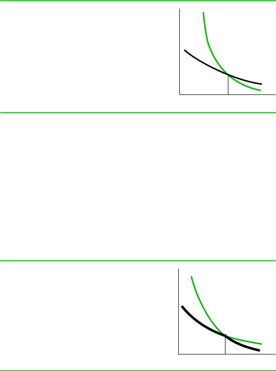
Contrast this with the training and skills of a thoracic surgeon. Thoracic surgeons specialize in the thoracic region, between the neck and the abdomen. To become a thoracic surgeon, a medical school graduate must complete a residency in general surgery and then an additional two-year residency in thoracic surgery. Figure 2.5 depicts average “cost” curves for thoracic surgery performed by a general surgeon and a thoracic surgeon. We use “cost” in quotes because it represents the full cost of care, which is lower if the surgery is successful. (Successful surgery usually implies fewer complications, shorter hospital
stays, and a shorter period of recuperation.) The average cost curves are downward sloping to reflect the spreading out of the initial investments in training. The cost curve for the thoracic surgeon starts off much higher than the cost curve for the general surgeon because of the greater investment in time. However, the thoracic surgeon’s cost curve eventually falls below the cost curve of a general surgeon because the thoracic surgeon will perform thoracic surgery more effectively than most general surgeons.
According to Smith’s theorem, when the demand for thoracic surgery in a market is low, then the market will not support a specialized surgeon. Instead, thoracic surgery will be performed by a general surgeon, who may also perform other kinds of surgery. This may be seen in Figure 2.6, which superimposes demand curves over cost curves. For low levels of demand, such as at D1, the market can support a general surgeon. A general surgeon who charges a price for thoracic surgery above P1 can more than cover average costs. When demand is D1, the market cannot support a thoracic surgeon. There is no price high enough to enable thoracic surgeons to recoup their costs.
FIGURE 2.5
Cost Curves for General and Thoracic Surgeons
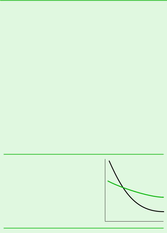
General surgeons incur lower training costs than do thoracic surgeons but are usually less efficient in performing thoracic surgery. Thus, the general surgeon’s average cost curve is below the thoracic surgeon’s for low volumes (reflecting lower average fixed costs) but above the thoracic surgeon’s for high volumes (reflecting higher average variable costs).
Average cost
General
Surgeons
Thoracic
Surgeons
Quantity of surgeries