

16 • Economics Primer: Basic Principles
•When average cost is an increasing function of output, marginal cost is greater than average cost.
These relationships follow from the mathematical properties of average and marginal cost, but they are also intuitive. If the average of a group of things (costs of manufacturing cellular phones, test scores, or whatever) increases when one more thing (one more phone, one more test) is added to the group, then it must be because the value of the most recently added thing—the “marginal”—is greater than the average. Conversely, if the average falls, it must be because the marginal is less than the average.
The Importance of the Time Period: Long-Run versus Short-Run Cost Functions
We emphasized the importance of the time horizon when discussing fixed versus variable costs. In this section, we develop this point further and consider some of its implications.
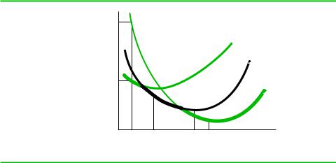
Figure P.6 illustrates the case of a firm whose production can take place in a facility that comes in three different sizes: small, medium, and large. Once the firm commits to a production facility of a particular size, it can vary output only by varying the quantities of inputs other than the plant size (e.g., by hiring another shift of workers). The period of time in which the firm cannot adjust the size of its production facilities is known as the short run. For each plant size, there is an associated short-run average cost function, denoted by SAC. These average cost functions include the annual costs of all relevant variable inputs (labor, materials) as well as the fixed cost (appropriately annualized) of the plant itself.
If the firm knows how much output it plans to produce before building a plant, then to minimize its costs, it should choose the plant size that results in the lowest
FIGURE P.6
Short-Run and Long-Run Average Cost Functions
Average cost
SACL(Q1)
SACS(Q1)
SACS(Q)
SACM(Q)
SACL(Q)
Q1 Q2 |
Q3 Q4 |
|
Q Output |
The curves labeled SACS(Q), SACM(Q), and SACL(Q) are the short-run average cost functions associated with small, medium, and large plants, respectively. For any level of output, the optimal plant size is the one with the lowest average cost. For example, at output Q1, the small plant is best. At output Q2, the medium plant is best. At output Q3, the large plant is best. The long-run average cost function is the “lower envelope” of the short-run average cost functions, represented by the bold line. This curve shows the lowest attainable average cost for any output when the firm is free to adjust its plant size optimally.

Costs • 17
short-run average cost for that desired output level. For example, for output Q1, the optimal plant is a small one; for output Q2, the optimal plant is a medium one; for output Q3, the optimal plant is a large one. Figure P.6 illustrates that for larger outputs, the larger plant is best; for medium-output levels, the medium plant is best; and for small-output levels, the small plant is best. For example, when output is Q1, the reduction in average cost that results from switching from a large plant to a small plant is SACL(Q1) 2 SACS(Q1). This saving not only arises from reductions in the fixed costs of the plant, but also because the firm can more efficiently tailor the rest of its operations to its plant size. When the firm produces Q1 in the large plant, it may need to utilize more labor to assure steady materials flows within the large facility. The small plant may allow flows to be streamlined, making such labor unnecessary.
The long-run average cost function is the lower envelope of the short-run average cost functions and is depicted by the bold line in Figure P.6. It shows the lowest attainable average cost for any particular level of output when the firm can adjust its plant size optimally. This is the average cost function the firm faces before it has committed to a particular plant size.
In this example, the long-run average cost function exhibits economies of scale. By operating with larger plant sizes, the firm can lower its average costs. This raises a deceptively simple but extremely significant point. To realize the lower average costs, the firm must not only build a large plant but must also achieve sufficient output, so that the large plant is indeed the optimal one. It would be disastrous for the firm to build a large plant if it only achieved an output of, say, Q1. The firm would be saddled with an expensive underutilized facility. If we were to observe a firm in this situation, we might be tempted to conclude that the scale economies inherent in the production process were limited or nonexistent. This would be incorrect. Scale economies exist, but the firm is not selling enough output needed to exploit them. These concepts are closely tied to the concept of throughput that we introduce in Chapter 1. Essentially, firms cannot fully exploit economies of scale unless they have sufficient inputs for production and distribution to get their products to market. Without such throughput, strategies that hinge on scale economies are doomed to fail.
It is often useful to express short-run average costs as the sum of average fixed costs (AFC) and average variable costs (AVC):
SAC(Q) 5 AFC(Q) 1 AVC(Q)
Average fixed costs are the firm’s fixed costs (i.e., the annualized cost of the firm’s plant plus expenses, such as insurance and property taxes, that do not vary with the volume of output) expressed on a per-unit-of-output basis. Average variable costs are the firm’s variable costs (e.g., labor and materials) expressed on a per-unit-of-output basis. For example, suppose the firm’s plant has an annualized cost of $9 million and other annual fixed expenses total $1 million. Moreover, suppose the firm’s variable costs vary with output according to the formula 4Q2. Then we would have
AFC(Q) 5 10Q
AFC(Q) 5 4Q
AFC(Q) 5 10Q 1 4Q
Note that as the volume of output increases, average fixed costs become smaller, which tends to pull down SAC. Average fixed costs decline because total fixed costs are being
18 • Economics Primer: Basic Principles
spread over an ever-larger production volume. Offsetting this (in this example) is the fact that average variable costs rise with output, which pulls SAC upward. The net effect of these offsetting forces creates the U-shaped SAC curves in Figure P.6.
Sunk versus Avoidable Costs
When assessing the costs of a decision, the manager should consider only those costs that the decision actually affects. Some costs must be incurred no matter what the decision is and thus cannot be avoided. These are called sunk costs. The opposite of sunk costs is avoidable costs. These costs can be avoided if certain choices are made. When weighing the costs of a decision, the decision maker should ignore sunk costs and consider only avoidable costs.
To illustrate the concept of sunk costs, take the case of an online merchandiser of laser printers. The merchandiser traditionally purchased large quantities of printers from the manufacturer, so that it could satisfy rush orders. Increasingly, though, the merchandiser was carrying high inventories, including some lines that the manufacturer no longer produced and would not repurchase. A natural response to this problem would be to put the discontinued lines on sale and reduce inventory. However, the firm’s managers were reluctant to do this. They felt that even in the best of times the margins on their products barely covered their overhead, and by cutting the price, they would be unable to cover their cost of the goods they sold.
This argument is wrong. The cost incurred to purchase the laser printers is a sunk cost as far as pricing is concerned. Whether or not the merchandiser cuts price, it cannot avoid these costs. If it believes that a seller should never price below average cost, the merchandiser will end up with large losses. Instead, it should accept that it cannot undo past decisions (and their associated sunk costs) and strive to minimize its losses.
It is important to emphasize that whether a cost is sunk depends on the decision being made and the options at hand. In the example just given, the cost of the discontinued lines of printers is a sunk cost with respect to the pricing decision today. But before the printers were ordered, their cost would not have been sunk. By not ordering them, the merchandiser would have avoided the purchase and storage costs.
Students often confuse sunk costs with fixed costs. The two concepts are not the same. In particular, some fixed costs need not be sunk. For example, a railroad serving Sydney to Adelaide needs a locomotive and a crew whether it hauls 1 carload of freight or 20. The cost of the locomotive is thus a fixed cost. However, it is not necessarily sunk. If the railroad abandons its Sydney to Adelaide line, it can sell the locomotive to another railroad or redeploy it to another route.
Sunk costs are important for the study of strategy, particularly in analyzing rivalry among firms, entry and exit decisions from markets, and decisions to adopt new technologies. For example, the concept of sunk costs helps explain why established American steel firms were unwilling to invest continuous casting technology, even as new Japanese firms building “greenfield” facilities did adopt the new technology. The new technology had higher fixed costs, but lower variable operating costs. Established American firms viewed the fixed cost of their old technologies as sunk. Thus, they compared the savings in operating costs against the fixed cost of the new technology. The Japanese firms, in contrast, compared the savings in operating costs against the difference between the fixed costs of the new and old technologies. American firms thus required a larger cost savings than the Japanese firms to induce them to adopt the new technology. Despite criticism in the popular business press, the American firms’