

28 • Economics Primer: Basic Principles
PERFECT COMPETITION
A special case of the theory of the firm is the theory of perfect competition. This theory highlights how market forces shape and constrain a firm’s behavior and interact with the firm’s decisions to determine profitability. The theory deals with a stark competitive environment: an industry with many firms producing identical products (so that consumers choose among firms solely on the basis of price) and where firms can enter or exit the industry at will. This is a caricature of any real market, but it does approximate industries such as aluminum smelting and copper mining in which many firms produce nearly identical products.
Because firms in a perfectly competitive industry produce identical products, each firm must charge the same price. This market price is beyond the control of any individual firm; it must take the market price as given. For a firm to offer to sell at a price above the market price would be folly because it would make no sales. Offering to sell below the market price would also be folly because the firm would needlessly sacrifice revenue. As shown in Figure P.11, then, a perfectly competitive firm’s demand curve is perfectly horizontal at the market price, even though the industry demand curve is downward sloping. Put another way, the firm-level price elasticity of demand facing a perfect competitor is infinite, even though the industry-level price elasticity is finite.
Given any particular market price, each firm must decide how much to produce. Applying the insights from the theory of the firm, the firm should produce at the point where marginal revenue equals marginal cost. When the firm’s demand curve is horizontal, each additional unit it sells adds sales revenue equal to the market price. Thus, the firm’s marginal revenue equals the market price, and the optimal output, shown in Figure P.11, is where marginal cost equals the market price. If we were to graph how a firm’s optimal output changed as the market price changed, we would trace out a curve that is identical to the firm’s marginal cost function. This is known as the firm’s supply curve. It shows the amount of output the perfectly competitive firm would sell at various market prices. Thus, the supply curve of a perfectly competitive firm is identical to its marginal cost function.
If we aggregate over the firm supply curves of all active producers in the industry, we get the industry supply curve, depicted in Figure P.12 as SS. This figure
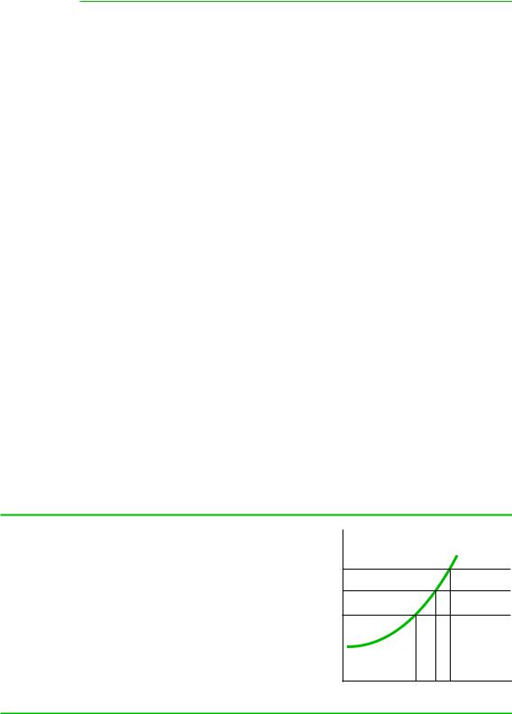
FIGURE P.11
Demand and Supply Curves for a Perfectly Competitive Firm
A perfectly competitive firm takes the market price |
|
|
as given and thus faces a horizontal demand curve at |
cost |
P2 |
the market price. This horizontal line also represents |
||
equals marginal cost. When the market price is P0, |
marginal |
P0 |
the firm’s marginal revenue curve MR. The firm’s |
|
P1 |
optimal output occurs where its marginal revenue |
|
|
the optimal output is Q0. If the market price were to |
Price, |
|
change, the firm’s optimal quantity would also |
|
|
|
|
change. At price P1, the optimal output is Q1. At price P0, the optimal output is Q0. The firm’s supply curve traces out the relationship between the market price and the firm’s optimal quantity of output. This curve is identical to the firm’s marginal cost curve.
MC
Price = MR
Q0 Q1 Q2
Q Quantity
Perfect Competition • 29
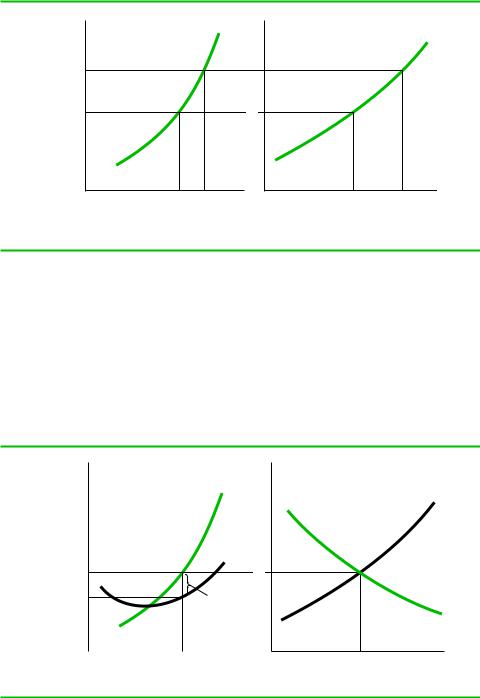
FIGURE P.12
Firm and Industry Supply Curves Under Perfect Competition
Price, marginal cost
$15
$10
MC
SS
Price
40 |
50 |
40,000 |
50,000 |
units |
units |
units |
units |
Firm’s quantity |
Industry quantity |
||
A single firm’s supply curve is shown in the graph on the left. The industry’s supply curve SS is shown in the graph on the right. These graphs depict an industry of 1,000 identical firms. Thus, at any price the industry supply is 1,000 times the amount that a single firm would supply.
shows an industry with 1,000 identical active firms. At any price, the industry supply is 1,000 times the supply of an individual firm. Given the industry supply curve, we can now see how the market price is determined. For the market to be in equilibrium, the market price must be such that the quantity demanded equals the quantity supplied by firms in the industry. This situation is depicted in Figure P.13, where
FIGURE P.13
Perfectly Competitive Industry Prior to New Entry
Price, marginal cost, average cost
MC
|
|
|
AC |
P* |
|
|
|
AC(q*) |
|
|
Profit |
|
|
||
|
|
||
|
|
|
per unit |
|
|
|
|
|
q* |
||
|
Firm’s quantity |
||
SS
Price
D
Q*
Industry quantity
At the price P*, each firm is producing its optimal amount of output q*. Moreover, the quantity demanded equals the quantity Q* supplied by all firms in the industry. However, each firm is earning a positive profit because at q*, the price P* exceeds average cost AC(q*), resulting in a profit on every unit sold. New firms would thus want to enter this industry.
30 • Economics Primer: Basic Principles
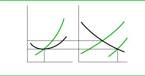
FIGURE P.14
Perfectly Competitive Industry at Long-Run Equilibrium
Price, marginal cost, average cost
P*
P**
MC
AC
q**
Firm’s quantity
Price
SS
SS′
D
Q** Industry quantity
At price P*, new entrants are attracted to the industry. As they come in, the industry’s supply curve shifts to the right, from SS to SS9, resulting in a reduction in market price. Entry ceases to occur when firms are earning as much inside the industry as they can earn outside it. Each firm thus earns zero economic profit, or equivalently, price equals average cost. Firms are choosing the optimal output and earning zero economic profit when they produce at the point at which market price equals both marginal cost and average cost. This occurs when the price is P** and firms produce q**. Firms are thus at the minimum point on their average cost function.
P* denotes the price that “clears” the market. If the market price was higher than P*, then more of the product would be offered for sale than consumers would like to buy. The excess supply would then place downward pressure on the market price. If the market price was lower than P*, then there would be less of the product offered for sale than consumers would like to buy. Here, the excess demand would exert upward pressure on the market price. Only when the quantities demanded and supplied are equal—when price equals P*—is there no pressure on price to change.
The situation shown in Figure P.13 would be the end of the story if additional firms could not enter the industry. However, in a perfectly competitive industry, firms can enter and exit at will. The situation in Figure P.13 is thus unstable because firms in the industry are making a profit (price exceeds average cost at the quantity q* that each firm supplies). Thus, it will be attractive for additional firms to enter and begin selling. Figure P.14 shows the adjustment that occurs. As more firms enter, the supply curve SS shifts outward to SS9. As this happens, the quantity supplied exceeds the quantity demanded, and there is pressure on price to fall. It will continue to fall until no additional entry occurs. This is when the market price just equals a typical firm’s average cost. As we have seen, to optimize output, firms produce where market price equals marginal cost. Thus, in the longrun equilibrium depicted in Figure P.14, firms are producing at minimum efficient scale (recall, this is the quantity corresponding to the minimum point on the average cost curve), and the equilibrium market price P** equals the minimum level of average cost.
Suppose, now, that market demand suddenly falls. Figure P.15 shows what happens. The fall in market demand is represented by a shift from demand curve D0 to D1. Initially, market price would fall to P9, and firms’ revenues would not cover their economic costs. The industry “shakeout” then begins. Firms begin to exit the industry.