Добавил:

Upload Опубликованный материал нарушает ваши авторские права? Сообщите нам.

Вуз:

Челябинский Государственный Университет

Предмет:

[НЕСОРТИРОВАННОЕ]

Файл:

Eviews5 / EViews5 / Docs / EViews 5 Users Guide.pdf

Скачиваний:

152

Добавлен:

23.03.2015

Размер:

11.51 Mб

Скачать

☆

<<< < Предыдущая 85 86 87 88 89 90 91 92 93 94 95 9697 / 16697 98 99 100 101 102 103 104 105 106 107 108 109 > Следующая >>>

Procedures for Binary Equations—633

Dependent Variable: GRADE
Method: ML - Binary Probit
Date: 07/31/00		Time: 15:57
Sample: 1 32
Included observations: 32
Andrews and Hosmer-Lemeshow Goodness-of-Fit Tests
Grouping based upon predicted risk (randomize ties)

	Quantile of Risk			Dep=0		Dep=1	Total	H-L
	Low	High	Actual	Expect	Actual	Expect	Obs	Value

1	0.0161	0.0185	3	2.94722	0	0.05278	3	0.05372
2	0.0186	0.0272	3	2.93223	0	0.06777	3	0.06934
3	0.0309	0.0457	3	2.87888	0	0.12112	3	0.12621
4	0.0531	0.1088	3	2.77618	0	0.22382	3	0.24186
5	0.1235	0.1952	2	3.29779	2	0.70221	4	2.90924
6	0.2732	0.3287	3	2.07481	0	0.92519	3	1.33775
7	0.3563	0.5400	2	1.61497	1	1.38503	3	0.19883
8	0.5546	0.6424	1	1.20962	2	1.79038	3	0.06087
9	0.6572	0.8342	0	0.84550	3	2.15450	3	1.17730
10	0.8400	0.9522	1	0.45575	3	3.54425	4	0.73351

		Total	21	21.0330	11	10.9670	32	6.90863

H-L Statistic:			6.9086			Prob. Chi-Sq(8)		0.5465
Andrews Statistic:			20.6045			Prob. Chi-Sq(10)		0.0240

The columns labeled “Quantiles of Risk” depict the high and low value of the predicted probability for each decile. Also depicted are the actual and expected number of observations in each group, as well as the contribution of each group to the overall Hosmer-Leme- show (H-L) statistic—large values indicate large differences between the actual and predicted values for that decile.

The χ2 statistics are reported at the bottom of the table. Since grouping on the basis of the fitted values falls within the structure of an Andrews test, we report results for both the H- L and the Andrews test statistic. The p-value for the HL test is large while the value for the Andrews test statistic is small, providing mixed evidence of problems. Furthermore, the relatively small sample sizes suggest that caution is in order in interpreting the results.

Procedures for Binary Equations

In addition to the usual procedures for equations, EViews allows you to forecast the dependent variable and linear index, or to compute a variety of residuals associated with the binary model.

Forecast

EViews allows you to compute either the fitted probability, ˆ i p

ted values of the index xi′ β . From the equation toolbar select ability/Index)…, and then click on the desired entry.

=	ˆ
	1 − F( −xi′β) , or the fit-

Proc/Forecast (Fitted Prob-

As with other estimators, you can select a forecast sample, and display a graph of the forecast. If your explanatory variables, xt , include lagged values of the binary dependent vari-

pˆ t − 1

634—Chapter 21. Discrete and Limited Dependent Variable Models

able yt , forecasting with the Dynamic option instructs EViews to use the fitted values , to derive the forecasts, in contrast with the Static option, which uses the actual

(lagged) yt − 1 .

Neither forecast evaluations nor automatic calculation of standard errors of the forecast are currently available for this estimation method. The latter can be computed using the variance matrix of the coefficients displayed by View/Covariance Matrix, or using the

@covariance function.

You can use the fitted index in a variety of ways, for example, to compute the marginal effects of the explanatory variables. Simply forecast the fitted index and save the results in a series, say XB. Then the auto-series @dnorm(-xb), @dlogistic(-xb), or @dex- treme(-xb) may be multiplied by the coefficients of interest to provide an estimate of the derivatives of the expected value of yi with respect to the j-th variable in xi :

∂E( yi	xi, β)
------------------------------ = f( −xi′β) βj .		(21.14)
∂xij

Make Residual Series

Proc/Make Residual Series gives you the option of generating one of the following three types of residuals:

			Ordinary	eoi		ˆ
				eoi	= yi − pi
			Standardized			ˆ
				esi	=	y i − pi
				esi	=	-- -------------------------ˆ	ˆ
						p i ( 1 − pi)
			Generalized			ˆ	ˆ
				egi	=	( y i − p i ) f( −xi′β)		φ
				egi	=	------------------------------------------ˆ	ˆ	φ
						p i ( 1	− pi)
ˆ	=		ˆ
where pi	=	1 − F( − xi′β) is the fitted probability, and the distribution and density func-

tions F and f , depend on the specified distribution.

The ordinary residuals have been described above. The standardized residuals are simply the ordinary residuals divided by an estimate of the theoretical standard deviation. The generalized residuals are derived from the first order conditions that define the ML estimates. The first order conditions may be regarded as an orthogonality condition between the generalized residuals and the regressors x .

∂l( β)	=	N ( yi − ( 1 − F( −xi′β) ) ) f( − xi′β)		N
-------------∂β		Σ	---------------------------------------------------------------------------F ( − x i ′ β ) ( 1 − F ( − x i ′ β ) )	xi = Σ eg, i xi . (21.15)
		i = 1		i = 1

Procedures for Binary Equations—635

This property is analogous to the orthogonality condition between the (ordinary) residuals and the regressors in linear regression models.

The usefulness of the generalized residuals derives from the fact that you can easily obtain the score vectors by multiplying the generalized residuals by each of the regressors in x . These scores can be used in a variety of LM specification tests (see Chesher, Lancaster and Irish (1985), and Gourieroux, Monfort, Renault, and Trognon (1987)). We provide an example below.

Demonstrations

You can easily use the results of a binary model in additional analysis. Here, we provide demonstrations of using EViews to plot a probability response curve and to test for heteroskedasticity in the residuals.

Plotting Probability Response Curves

You can use the estimated coefficients from a binary model to examine how the predicted probabilities vary with an independent variable. To do so, we will use the EViews built-in modeling features.

For the probit example above, suppose we are interested in the effect of teaching method (PSI) on educational improvement (GRADE). We wish to plot the fitted probabilities of GRADE improvement as a function of GPA for the two values of PSI, fixing the values of other variables at their sample means.

We will perform the analysis using a grid of values for GPA from 2 to 4. First, we will create a series containing the values of GPA for which we wish to examine the fitted probabilities for GRADE. The easiest way to do this is to use the @trend function to generate a new series:

series gpa_plot=2+(4-2)*@trend/(@obs(@trend)-1)

@trend creates a series that begins at 0 in the first observation of the sample, and increases by 1 for each subsequent observation, up through @obs-1.

Next, we will use a model object to define and perform the desired computations. The following discussion skims over many of the useful features of EViews models. Those wishing greater detail should consult Chapter 26, “Models”, beginning on page 777.

636—Chapter 21. Discrete and Limited Dependent Variable Models

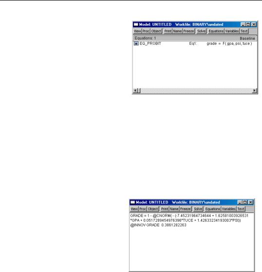
First, we create a model out of the estimated equation by selecting Proc/ Make Model from the equation toolbar. EViews will create an untitled model object containing a link to the estimated equation and will open the model window.

Next we want to edit this model specification so that calculations are performed using our simulation values. To

do so we must first break the link between the original equation and the model specification by selecting Proc/Links/Break All Links. Next, click on the Text button or select View/Source Text to display the text editing screen.

We wish to create two separate equations: one with the value of PSI set to 0 and one with the value of PSI set to 1 (you can, of course, use copy-and-paste to aid in creating the additional equation). We will also edit the specification so that references to GPA are replaced with the series of simulation values GPA_PLOT, and references to TUCE are replaced with the calculated mean, “@MEAN(TUCE)”. The GRADE_0 equation sets PSI to 0, while the GRADE_1 contains an additional expression, 1.426332342, which is the coefficient on the PSI variable.

Once you have edited your model, click on Solve and set the “Active” solution scenario to “Actuals”. This tells EViews that you wish to place the solutions in the series “GRADE_0” and “GRADE_1” as specified in the equation definitions. You can safely ignore the remaining solution settings and simply click on OK. EViews will report that your model has solved successfully.

You are now ready to plot results. Select Object/New Object.../Group, and enter:

gpa_plot grade_0 grade_1

EViews will open an untitled group window containing these two series. Select View/ Graph/XY line to display the probability of GRADE improvement plotted against GPA for those with and without PSI (and with the TUCE evaluated at means).

Procedures for Binary Equations—637

EViews will open a group window containing these series. Select View/Graph/XY line from the group toolbar to display a graph of your results.

We have annotated the graph slightly so that you can better judge the effect of the new teaching methods (PSI) on the GPA—Grade Improvement relationship.

Testing for Heteroskedasticity

As an example of specification tests
for binary dependent variable mod-
els, we carry out the LM test for het-
eroskedasticity using the artificial
regression method described by
Davidson and MacKinnon (1993,
section 15.4). We test the null
hypothesis of homoskedasticity
against the alternative of heteroskedasticity of the form:
var( ui) = exp ( 2zi′γ) ,	(21.16)

where γ is an unknown parameter. In this example, we take PSI as the only variable in z . The test statistic is the explained sum of squares from the regression:

′

( y i − p i )

f ( − xi′ β)

f( −xi′β) ( −xi

′β)

′b

2 + vi ,

(21.17)

-- ------------------------- ˆ

( 1

-- -------------------------ˆ

xib1

------------------------------------ˆ

----- zi

p i

− pi)

p i ( 1

− pi)

pi( 1

− pi)

which is asymptotically distributed as a χ2 with degrees of freedom equal to the number of variables in z (in this case 1).

ˆ	and fitted index xi′β .
To carry out the test, we first retrieve the fitted probabilities pi

Click on the Forecast button and first save the fitted probabilities as P_HAT and then the index as XB (you will have to click Forecast twice to save the two series).

Next, the dependent variable in the test regression may be obtained as the standardized residual. Select Proc/Make Residual Series… and select Standardized Residual. We will save the series as BRMR_Y.

Lastly, we will use the built-in EViews functions for evaluating the normal density and cumulative distribution function to create a group object containing the independent variables:

series fac=@dnorm(-xb)/@sqrt(p_hat*(1-p_hat))

group brmr_x fac (gpa*fac) (tuce*fac) (psi*fac)

<<< < Предыдущая 85 86 87 88 89 90 91 92 93 94 95 9697 / 16697 98 99 100 101 102 103 104 105 106 107 108 109 > Следующая >>>

Соседние файлы в папке Docs

#
23.03.20155.23 Mб47EViews 5 Command Ref.pdf
#
23.03.201511.51 Mб152EViews 5 Users Guide.pdf