

Chapter 3. Workfile Basics
Managing the variety of tasks associated with your work can be a complex and timeconsuming process. Fortunately, EViews’ innovative design takes much of the effort out of organizing your work, allowing you to concentrate on the substance of your project. EViews provides sophisticated features that allow you to work with various types of data in an intuitive and convenient fashion.
Before describing these features, we begin by outlining the basic concepts underlying the EViews approach to working with datasets using workfiles, and describing simple methods to get you started on creating and working with workfiles in EViews.
What is a Workfile?
At a basic level, a workfile is simply a container for EViews objects (see Chapter 4, “Object Basics”, on page 73). Most of your work in EViews will involve objects that are contained in a workfile, so your first step in any project will be to create a new workfile or to load an existing workfile into memory.
Every workfile contains one or more workfile pages, each with its own objects. A workfile page may be thought of as a subworkfile or subdirectory that allows you to organize the data within the workfile.
For most purposes, you may treat a workfile page as though it were a workfile (just as a subdirectory is also a directory) since there is often no practical distinction between the two. Indeed, in the most common setting where a workfile contains only a single page, the two are completely synonymous. Where there is no possibility of confusion, we will use the terms “workfile” and “workfile page” interchangeably.
Workfiles and Datasets
While workfiles and workfile pages are designed to hold a variety of EViews objects, such as equations, graphs, and matrices, their primary purpose is to hold the contents of datasets. A dataset is defined here as a data rectangle, consisting of a set of observations on one or more variables—for example, a time series of observations on the variables GDP, investment, and interest rates, or perhaps a random sample of observations containing individual incomes and tax liabilities.
Key to the notion of a dataset is the idea that each observation in the dataset has a unique identifier, or ID. Identifiers usually contain important information about the observation, such as a date, a name, or perhaps an identifying code. For example, annual time series data typically use year identifiers (“1990”, “1991”, ...), while

50—Chapter 3. Workfile Basics
cross-sectional state data generally use state names or abbreviations (“AL”, “AK”, ..., “WY”). More complicated identifiers are associated with longitudinal data, where one typically uses both an individual ID and a date ID to identify each observation.
Observation IDs are often, but not always, included as a part of the dataset. Annual datasets, for example, usually include a variable containing the year associated with each observation. Similarly, large cross-sectional survey data typically include an interview number used to identify individuals.
In other cases, observation IDs are not provided in the dataset, but external information is available. You may know, for example, that the 21 otherwise unidentified observations in a dataset are for consecutive years beginning in 1990 and continuing to 2010.
In the rare case were there is no additional identifying information, one may simply use a set of default integer identifiers that enumerate the observations in the dataset (“1”, “2”, “3”, ...).
Since the primary purpose of every workfile page is to hold the contents of a single dataset, each page must contain information about observation identifiers. Once identifier information is provided, the workfile page provides context for working with observations in the associated dataset, allowing you to use dates, handle lags, or work with longitudinal data structures.
Creating a Workfile
There are several ways to create and set up a new workfile. The first task you will face in setting up a workfile (or workfile page) is to specify the structure of your workfile. We focus here on three distinct approaches:
First, you may simply describe the structure of your workfile. EViews will create a new workfile for you to enter or import your data.
Describing the workfile is the simplest method, requiring only that you answer a few simple questions—it works best when the identifiers follow a simple pattern that is easily described (for example, “annual data from 1950 to 2000” or “quarterly data from 1970Q1 to 2002Q4”). This approach must be employed if you plan to enter data into EViews by typing or copy-and-pasting data.
In the second approach, you simply open and read data from a foreign data source. EViews will analyze the data source, create a workfile, and then automatically import your data.
The final approach, which should be reserved for more complex settings, involves two distinct steps. In the first, you create a new workfile using one of the first two approaches (by describing the structure of the workfile, or by opening and reading from a foreign data
Creating a Workfile—51
source). Next, you will structure the workfile, by showing EViews how to construct unique identifiers, in some cases by using values of the variables contained in the dataset.
We begin by describing the first two methods. The third approach, involving the more complicated task of structuring a workfile, will be taken up in “Structuring a Workfile” on page 207.
Creating a Workfile by Describing its Structure
To describe the structure of your workfile, you will need to provide EViews with external information about your observations and their associated identifiers. As examples, you might tell EViews that your dataset consists of a time series of observations for each quarter from 1990Q1 to 2003Q4, or that you have information for every day from the beginning of 1997 to the end of 2001, or that you have a dataset with 500 observations and no additional identifier information.
To create a new workfile, select File/New Workfile... from the main menu to open the
Workfile Create dialog.
On the left side of the dialog is a combo box for describing the underlying structure of your dataset. You will choose between the Dated - regular frequency, the Unstructured, and the Balanced Panel settings. Generally speaking, you should use Dated - regular frequency if you have a simple time series dataset, for a simple panel dataset you should use Balanced Panel, and in all other cases, you should select Unstructured. Additional detail to aid you in making a selection is provided in the description of each category.
Describing a Dated Regular Frequency
Workfile
When you select Dated - regular frequency, EViews will prompt you to select a frequency for your data. You may choose between the standard EViews supported date frequencies (Annual, Semi-annual,
Quarterly, Monthly, Weekly, Daily - 5 day week, Daily - 7 day week), and a special frequency (Integer date) which is a generalization of a simple enumeration.
In selecting a frequency, you set intervals between observations in your data (whether they are annual, semi-annual, quarterly, monthly, weekly, 5-day daily, or 7-day daily), which allows EViews to use all available calendar information to organize and manage your data. For example, when moving between daily and weekly or annual data, EViews knows that some years contain days in each of 53 weeks, and that some years have 366 days, and will use this information when working with your data.

52—Chapter 3. Workfile Basics
As the name suggests, regular frequency data arrive at regular intervals, defined by the specified frequency (e.g., monthly). In contrast, irregular frequency data do not arrive in regular intervals. An important example of irregular data is found in stock and bond prices where the presence of holidays and other market closures ensures that data are observed only irregularly, and not in a regular 5-day daily frequency. Standard macroeconomic data such as quarterly GDP or monthly housing starts are examples of regular data.
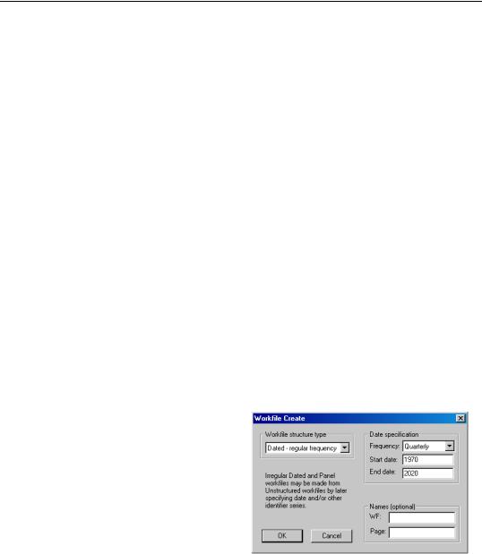
EViews also prompts you to enter a Start date and End date for your workfile. When you click on OK, EViews will create a regular frequency workfile with the specified number of observations and the associated identifiers.
Suppose, for example, that you wish to create a quarterly workfile that begins with the first quarter of 1970 and ends in the last quarter of 2020.
•First, select Dated - regular frequency for the workfile structure, and then choose the Quarterly frequency.
•Next, enter the Start date and End date. There are a number of ways to fill in the dates. EViews will use the largest set of observations consistent with those dates, so if you enter “1970” and “2020”, your quarterly workfile will begin in the first quarter of 1970, and end in the last quarter of 2020. Entering the date pair “Mar 1970” and “Nov 2020”, or the start-end pair “3/2/1970” and “11/15/2020” would have generated a workfile with the same structure, since the implicit start and end quarters are the same in all three cases.
This latter example illustrates a fundamental principle regarding the use of date information in EViews. Once you specify a date frequency for a workfile, EViews will use all available calendar information when interpreting date information. For example, given a quarterly frequency workfile, EViews knows that the date “3/2/1990” is in the first quarter of 1990 (see “Dates” on page 129 of the Command and Programming Reference for details).
Lastly, you may optionally provide a name to be given to your workfile and a name to be given to the workfile page.
Describing an Unstructured Workfile
Unstructured data are simply undated data which use the default integer identifiers. You should choose the Unstructured type if you wish to create a workfile that uses the default identifiers, or if your data are not a Dated - regular frequency or Balanced Panel.

Creating a Workfile—53
When you select this structure in the combo box, the remainder of the dialog will change, displaying a single field prompting you for the number of observations. Enter the number of observations, and click on OK to proceed. In the example depicted here, EViews will create a 500 observation workfile containing integer identifiers ranging from 1 to 500.
In many cases, the integer identifiers will be sufficient for you to work with your data. In more complicated settings, you may wish to further refine your identifiers. We describe this process in “Applying a Structure to a Workfile” on page 218.
Describing a Balanced Panel Workfile
The Balanced Panel entry provides a simple method of describing a regular frequency panel data structure. Panel data is the term that we use to refer to data containing observations with both a group (cross-section) and cell (within-group) identifiers.
This entry may be used when you wish to create a balanced structure in which every cross-section follows the same regular frequency with the same date observations. Only the barest outlines of the procedure are provided here since a proper discussion requires a full description of panel data and the creation of the advanced workfile structures. Panel data and structured workfiles are discussed at length in “Structuring a Workfile” on
page 207.
To create a balanced panel, select Balanced Panel in the combo box, specify the desired Frequency, and enter the
Start date and End date, and Number of cross sections. You may optionally name the workfile and the workfile page. Click on OK. EViews will create a balanced panel workfile of the given frequency, using the specified start and end dates and number of cross-sections.
Here, EViews creates a 200 cross-section, regular frequency, quarterly panel workfile with observations beginning in 1970Q1 and ending in 2020Q4.
Unbalanced panel workfiles or workfiles involving more complex panel structures should be created by first defining an unstructured workfile, and then applying a panel workfile structure.
Creating a Workfile by Reading from a Foreign Data Source
A second method of creating an EViews workfile is to open a foreign (non-EViews format) data source and to read the data into an new EViews workfile.

54—Chapter 3. Workfile Basics
The easiest way to read foreign data into a new workfile is to copy the foreign data source to the Windows clipboard, right click on the gray area in your EViews window, and select Paste as new Workfile. EViews will automatically create a new workfile containing the contents of the clipboard. Such an approach, while convenient, is only practical for small amounts of data.
Alternately, you may open a foreign data source as an EViews workfile. To open a foreign data source, first select File/Open/Foreign Data as Workfile..., to bring up the standard file Open dialog. Clicking on the Files of type combo box brings up a list of the file types that EViews currently supports for opening a workfile.
If you select a time series database file (Aremos TSD, GiveWin/Pc-Give, Rats 4.x, Rats Portable, TSP Portable), EViews will create a new, regular frequency workfile containing the contents of the entire file. If there are mixed frequencies in the database, EViews will select the lowest frequency, and convert all of the series to that frequency using the default conversion settings (we emphasize here that all of these database formats may also be opened as databases by selecting File/Open/Database... and filling out the dialogs, allowing for additional control over the series to be read, the new workfile frequency, and any frequency conversion).
If you choose one of the remaining source types, EViews will create a new unstructured workfile. First, EViews will open a series of dialogs prompting you to describe and select data to be read. The data will be read into the new workfile, which will be resized to fit. If there is a single date series in the data, EViews will attempt to restructure the workfile using the date series. If this is not possible but you still wish to use dates with these data, you will have to define a structured workfile using the advanced workfile structure tools (see “Structuring a Workfile” beginning on page 207).
The import as workfile interface is available for Microsoft Access files, Gauss Dataset files, ODBC Dsn files, ODBC Query files, SAS Transport files, native SPSS files (using the SPSS Input/output .DLL that should be installed on your system), SPSS Portable files, Stata files, Excel files, raw ASCII or binary files, or ODBC Databases and queries (using the ODBC driver already present on your system).
An Illustration
We will use a Stata file to illustrate the basic process of creating a new workfile (or a workfile page) by opening a foreign source file.

Creating a Workfile—55
To open the file, first navigate to the appropriate directory and select Stata file to display available files of that type. Next, double-click on the name to select and open the file, or enter the filename in the dialog and click on Open to accept the selection.
A simple alternative to opening the file from the menu is to drag-and-drop your foreign file into the EViews window.
EViews will open the selected file, validate its type, and will display a tabbed dialog allowing you to select the specific data that you wish to read into your
new workfile. If you wish to read all of your data using the default settings, click on OK to proceed. Otherwise you may use each of the tabs to change the read behavior.
The Select variables tab of the dialog should be used to choose the series data to be included. The upper list box shows the names of the variables that can be read into EViews series, along with the variable data type, and if available, a description of the data. The variables are first listed in the order in which they appear in the file. You may choose to sort the data by clicking on the header for the column. The display will be toggled between three states: the original order, sorted (ascending), and sorted (descending). In the latter two cases, EViews will display a

56—Chapter 3. Workfile Basics
small arrow on the header column indicating the sort type. Here, the data are sorted by variable name in ascending order.
When the dialog first opens, all variables are selected for reading. You can change the current state of any variable by checking or unchecking the corresponding checkbox. The number of variables selected is displayed at the bottom right of the list.
There may be times when checking and unchecking individual variables is inconvenient (e.g., when there are thousands of variable names). The bottom portion of the dialog provides you with a control that allows you to select or unselect variables by name. Simply enter the names of variables using wildcard characters if desired, choose the types of interest, and click on the appropriate button. For example, entering “A* B?” in the selection edit box, selecting only the Numeric checkbox, and clicking on Unselect will uncheck all numeric series beginning with the letter “A” and all numeric series with two character names beginning in “B”.
When opening datasets that contain value labels, EViews will display a second tabbed dialog page labeled Select maps, which controls the importing of value maps. On this page, you will specify how you wish EViews to handle these value labels. You should bear in mind that when opening datasets which do not contain value labels, EViews will not display the value map tab.
The upper portion of the dialog contains a combo box where you specify which labels to read. You may choose between the default
Attached to selected series, None, All, or Selected from list.
The selections should be self-
explanatory—Attached to selected series will only load maps that are used by the series that you have selected for inclusion; Selected from list (depicted) displays a map selection list in which you may check and uncheck individual label names along with a control to facilitate selecting and deselecting labels by name.