EViews objects (series, groups, equations, and so on) display their views as graphs, tables, and text. You may, for example, display the descriptive statistics of a set of series or the regression output from an equation as a table, or the impulse responses from a VAR as a graph.
While object views may be customized in limited fashion, the customization is generally transitory. When you close the object and redisplay the view, most customized settings will be lost. Moreover, since views are often dynamic, when the underlying object changes, or the active sample changes, so do the object views.
One may wish to preserve the current view, along with any customization, so that it does not change when the object changes. In EViews, this action is referred to as freezing the view. Freezing a view will create a new object containing a “snapshot” of the current contents of the view window. The type of object created varies with the original view: freezing a graphical view creates a graph object, freezing a tabular view creates a table object, and freezing a text view creates a text object.
Frozen views form the basis of most presentation output, and EViews provides tools for customizing the appearance of these objects. This chapter describes the options available for controlling the appearance of graph, table, and text objects.
Creating Graphs
Graph objects are usually created by freezing a view. Simply press the Freeze button in an object window which contains a graph view.
It is important to keep in mind the distinction between a graphical view of an object such as a series or a group, and a graph object created by freezing that view.
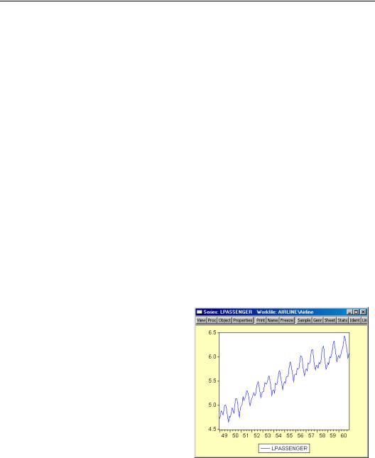
For example, suppose you wish to create a graph object containing a line graph of the series LPASSENGER. To display the line graph view of the series, select
View/Graph/Line from the LPASSENGER series menu. Notice the “Series: LPASSENGER” designation in the window titlebar that shows this is a view of the series object.
416—Chapter 14. Graphs, Tables, and Text Objects
You may customize this graph view in any of the ways described in “Customizing a Graph” on page 64 of the Command and Programming Reference, but these changes will be lost when the view is redrawn, e.g. when the object window is closed and reopened, when the workfile sample is modified, or when the data underlying the object are changed. If you would like to keep a customized graphical view, say for presentation purposes, you should create a graph object from the view.
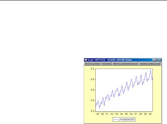
To create a graph object from the view, click on the Freeze button. EViews will create an UNTITLED graph object containing a snapshot of the view.
Here, the titlebar shows that we have an untitled graph object. The contents of the two windows are identical, since the graph object contains a copy of the contents of the original series view.
Notice also that since we are working with a graph object, the menubar provides access to a new set of views and procedures which allow you to further modify the contents of the graph object.
As with other EViews objects, the UNTITLED graph will not be saved
with the workfile. If you wish to store the frozen graph object in your workfile, you must name the graph object; press the Name button and provide a name.
You may also create a graph object by combining two or more existing named graph objects. Simply select all of the desired graphs and then double click on any one of the highlighted names. EViews will create a new, untitled graph, containing all of the selected graphs. An alternative method of combining graphs is to select Quick/Show… and enter the names of the graphs.
Modifying Graphs
A graph object is made up of a number of elements: the plot area, the axes, the graph legend, and one or more pieces of added text or shading. To select one of these elements for editing, simply click in the area associated with it. A blue box will appear around the selected element. Once you have made your selection, you can click and drag to move the element around the graph, or double click to bring up a dialog of options associated with the element.
Modifying Graphs—417
Alternatively, you may use the toolbar or the right mouse button menus to customize your graph. For example, clicking on the graph and then pressing the right mouse button brings up a menu containing tools for modifying and saving the graph.
The main options dialog may be opened by selecting Options...
from the right mouse menu. You may also double click anywhere in the graph window to bring up the Graph Options tabbed dia-
log. If you double-click on an applicable graph element (the legend, axes, etc.), the dialog will open to the appropriate tab.
Graph Types
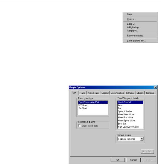
You may use the Graph Options dialog to customize your graph object. For most graphs, the Type tab allows you to change the graph type.
The listbox on the left-hand side of the Type tab provides access to the fundamental graph types. The listbox on the right will list the available graphs corresponding to the selected type. For example, if you select Time/Observation Plot on the left, the right-hand side listbox lists available time/observation graph types.
The fundamental graph types available depend on whether the graph involves a single series (or column of data) or more than one series (or col-
umn). For example, the Mixed Area & Line, Mixed Bar & Line, Mixed Spike & Line,
Error Bar, and High-Low(Open-Close)types are only available for graphs containing multiple series or matrix columns.
Note also that a number of statistical graphs do not allow you to change the graph type. In this case, either the Type tab will be unavailable, or the Basic graph type will be set to
Special.
Most of the graph types are self-explanatory, but a few comments may prove useful.
418—Chapter 14. Graphs, Tables, and Text Objects
If you select the Line & Symbol or Spike & Symbol type, you should use the Lines & Symbols tab to control the line pattern and/or symbol type. For area graphs, bar graphs, and pie charts, use the Filled Areas tab to control its appearance.
The Error Bar type is designed for displaying statistics with standard errors bands. This graph type shows a vertical error bar connecting the values for the first and second series. If the first series value is below the second series value, the bar will have outside half-lines. The (optional) third series is plotted as a symbol.
The High-Low(Open-Close)type displays up to four series. Data from the first two series (the high-low values) will be connected as a vertical line, the third series (the open value) is drawn as a left horizontal half-line, and the fourth series (the close value) is drawn as a right horizontal half-line. This graph type is commonly used to display daily stock price data.
The Stack lines & bars option plots the series so that each line represents the sum of all preceding series. In other words, each series value is the vertical distance between each successive line. Note that if some (but not all) of the series have missing values, the sum will be cumulated with missing values replaced by zeros.
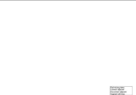
If your data includes sample breaks so that all of the observations in the graph are not consecutive, an additional pull-down menu will appear in the bottom right-hand portion of the tab, allowing you to
select how breaks are handled in the graph. You may, for example, choose to Pad the graph so that missing observations appear as blanks, or you may elect to connect the nonconsecutive graphs, with or without line segments showing the breaks (Segment with lines).
Once you have selected the graph type settings, click on Apply or OK to change the graph type. Selecting OK also closes the dialog.
Modifying Graphs—419
Basic Graph Characteristics
Underlying Graph Attributes
The Frame tab controls basic display characteristics of the graph, including color usage, framing style, indent position, grid lines.
You can also use this tab to control the aspect ratio of your graph using the predefined ratios, or you can input a custom set of dimensions. Note that the values are displayed in “virtual inches”.
Bear in mind that if have previously added text in the graph with user specified (absolute) position, changing the graph
frame size may change the relative position of the text in the graph.
To change or edit axes, select the Axes & Scaling tab. Depending on its type, a graph can have up to four axes: left, bottom, right, and top. Each series is assigned an axis as displayed in the upper right listbox.
You may change the assigned axis by first highlighting the series and then clicking on one of the available axis buttons. For example, to plot several series with a common scale, you should assign all series to the same axis. To plot
two series with a dual left-right scale, assign different axes to the two series.
420—Chapter 14. Graphs, Tables, and Text Objects
To edit characteristics of an axis, select the desired axis from the drop down menu at the top of the dialog; the left/right axes may be customized for all graphs. For the Time/ Observation Plot type, you may edit the bottom axis to control how the dates/observations are labeled. Alternately, for XY graphs, the bottom/top axes may be edited to control the appearance of the data scale.
To edit the graph legend characteristics, select the Legend tab. Note that if you place the legend using user specified (absolute) positions, the relative position of the legend may change when you change the graph frame size.
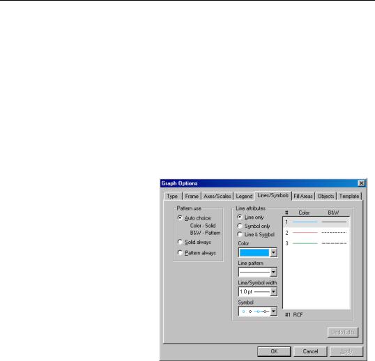
Data Display Attributes (Lines, Symbols, Filled Areas)
The Lines/Symbols tab provides you with control over the drawing of all lines and symbols corresponding to the data in your graph.
You may choose to display lines, symbols, or both, and you can customize the color, width, pattern, and symbol usage. See “Use of color with lines and filled areas” on page 65 of the Command and Programming Reference.
The current line and symbol settings will be displayed in the listbox on the right hand side of the dialog. Once you make your choices, click on Apply to see the effect of the new settings.
The Filled Areas tab allows
you to control the display characteristics of your area, bar, or pie graph. Here, you may customize the color, shading, and labeling of the graph elements.
Modifying Graphs—421
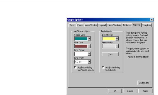
Added Text, Line, and Shade Attribute Defaults
The Objects tab allows you to control the default characteristics of new text, shade, or line drawing objects later added to the graph (see “Adding and Editing Text” on page 421 and “Adding Lines and Shades” on page 423).
You may select colors for the shade, line, box, or text box frame, as well as line patterns and widths, and text fonts and font characteristics.
By default, when you apply these changes to the graph object options, EViews will
update the default settings in the graph, and will use these settings when creating new line, shade, or text objects. Any existing lines, shades or text in the graph will not be updated. If you wish to modify the existing to use the new settings, you must check the
Apply to existing line/shade objects and Apply to existing text objects boxes prior to clicking on the Apply button.
Adding and Editing Text
You can customize a graph by adding one or more lines of text anywhere in the graph. This can be useful for labeling a particular observation or period, or for adding titles or remarks to the graph. To add new text, simply click on the AddText button in the toolbar or select
Proc/Add text…
422—Chapter 14. Graphs, Tables, and Text Objects
To modify an existing text object, simply double click on the object. The Text Labels dialog will be displayed.
Enter the text you wish to display in the large edit field. Spacing and capitalization (upper and lower case letters) will be preserved. If you want to enter more than one line, press the Enter key after each line.
•The Justification options determine how multiple lines will be aligned relative to each other.
•Font allows you to select a font and font characteristics for the text.
•Text in Box encloses the text in a box.
•Box fill color controls the color of the area inside the text box.
•Frame color controls the color of the frame of the text box.
The first four options in Position place the text at the indicated (relative) position outside the graph. You can also place the text by specifying its coordinates. Coordinates are set in virtual inches, with the origin at the upper left-hand corner of the graph.
The X-axis position increases as you move to the right of the origin, while the Y-axis increases as you move down from the origin. The default sizes, which are expressed in virtual inches, are taken from the global options, with the exception of scatter diagrams always default to 3 × 3 virtual inches.
Consider, for example, a graph with a size of 4 × 3 virtual inches. For this graph, the X=4, Y=3 position refers to the lower right
Modifying Graphs—423
hand corner of the graph. Labels will be placed with the upper left-hand corner of the enclosing box at the specified coordinate.
You can change the position of text added to the graph by selecting the text box and dragging it to the position you choose. After dragging to the desired position, you may double click on the text to bring up the Text Labels dialog to check the coordinates of that position or to make changes to the text. Note that if you specify the text position using coordinates, the relative position of the text may change when you change the graph frame size.
Adding Lines and Shades
You may draw lines or add a shaded area to the graph. From a graph object, click on the
Lines/Shade button in the toolbar or select Proc/Add shading…. The Lines & Shading dialog will appear:
Select whether you want to draw a line or add a shaded area, and enter the appropriate information to position the line or shaded area horizontally or vertically. If you select Vertical, EViews will prompt you to position the line or shaded area at a given observation. If you select Horizontal, you must provide a data value at which to draw the line or shaded area.
You should also use this dialog to choose a line pattern, width, and color for the line or shaded area, using the drop down menus.
If you check the Apply color... checkbox, EViews will update all of the existing lines or shades of the specified type in the graph.
To modify a single existing line or shaded area, simply double click on it to bring up the dialog.
Removing Graph Elements
To remove a graph element, simply select the element and press the Delete key. Alternately, you may select the element and then press the Remove button on the graph toolbar. For example, to remove text that you have placed on the graph, click on the text. A border will appear around the text. Press Delete or click on the Remove button to delete the text.
The same method may be applied to legends, scales, lines, or shading which have been added to the graph.
424—Chapter 14. Graphs, Tables, and Text Objects
Graph Templates
Having put a lot of effort into getting a graph to look just the way you want it, you may want to use the same options in another graph. EViews allows you to use any named graph as a template for a new or existing graph. You may think of a template as a graph style that can be applied to other graphs.
In addition, EViews provides a set of predefined templates that you may use to customize the graph. These predefined templates are not associated with objects in the workfile, and you are always available. The EViews templates provide easy-to-use examples of graph customization that may be applied to any graph. You may also find it useful to use the predefined templates as a foundation for your own graph template creation.
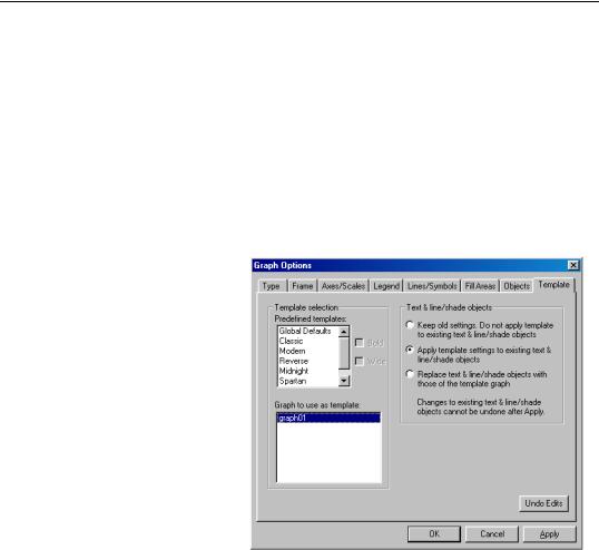
To update a graph using a template, double click on the graph area to display the
Graph Options dialog, and click on the Template tab. Alternatively, you may right mouse click, and select Template... to open the desired tab of the dialog.
On the left-hand side of the dialog you will first select your template. The upper list box contains a list of the EViews predefined templates. The lower list box contains a list of all of the named graphs in the current workfile page. Here,
we have selected the graph object GRAPH01 for use as our graph template.
If instead, you select one of the predefined templates, you will be given the choice of applying the Bold or Wide modifiers to the base template. As the name suggests, the Bold modifier changes the settings in the template so that lines and symbols are bolder (thicker, and larger) and adjusts other characteristics of the graph, such as the frame, to match. The Wide modifier changes the aspect ratio of the graph so that the horizontal to vertical ratio is increased.
You may reset the dialog by clicking on the Undo Edits button prior to clicking on Apply. When you click on the Apply button, EViews will immediately update all of the basic graph settings described in “Basic Graph Characteristics” on page 419, including graph size and aspect ratio, frame color and width, graph background color, grid line options, and