

Chapter 11. Series
EViews provides various statistical graphs, descriptive statistics, and procedures as views and procedures of a numeric series. Once you have read or generated data into series objects using any of the methods described in Chapter 5, “Basic Data Handling”, Chapter 6, “Working with Data”, and Chapter 10, “EViews Databases”, you are ready to perform statistical and graphical analysis using the data contained in the series.
Series views compute various statistics for a single series and display these statistics in various forms such as spreadsheets, tables, and graphs. The views range from a simple line graph, to kernel density estimators. Series procedures create new series from the data in existing series. These procedures include various seasonal adjustment methods, exponential smoothing methods, and the Hodrick-Prescott filter.
The group object is used when working with more than one series at the same time. Methods which involve groups are described in Chapter 12, “Groups”, on page 363.
To access the views and procedures for series, open the series window by double clicking on the series name in the workfile, or by typing show followed by the name of the series in the command window.
Series Views Overview
The series view drop-down menu is divided into four blocks. The first block lists views that display the underlying data in the series. The second and third blocks provide access to general statistics; the views in the third block are mainly for time series. The fourth block allows you to assign default series properties and to modify and display the series labels.
Spreadsheet and Graph Views
Spreadsheet
The spreadsheet view is the basic tabular view for the series data. Displays the raw, mapped, or transformed data series data in spreadsheet format.
You may customize your spreadsheet view extensively (see “Changing the Spreadsheet Display” in ”Data Objects” on page 88).
310—Chapter 11. Series
In addition, the right-mouse button menu allows you to write the contents of the spreadsheet view to a CSV, tab-delimited ASCII text, RTF, or HTML file. Simply right-mouse button click, select the Save table to disk... menu item, and fill out the resulting dialog.
Graph
The graph submenu contains entries for various types of basic graphical display of the series: Line, Area, Bar, Spike, Seasonal Stacked Line, Seasonal Split Line.
•Line plots the series against the date/observation number.
•Area is a filled line graph.
•Bar plots the bar graph of the series. This view is useful for plotting series from a small data set that takes only a few distinct values.
•Spike plots a spike graph of the series against the date/observation number. The spike graph depicts values of the series as vertical spikes from the origin.
•Seasonal Stacked Line and Seasonal Split Line plot the series against observations reordered by season. The seasonal line graph view is currently available only for quarterly and monthly frequency workfiles.
The stacked view reorders the series into seasonal groups where the first season observations are ordered by year, and then followed by the second season observations, and so on. Also depicted are the horizontal lines identifying the mean of the series in each season.
The split view plots the line graph for each season on an annual horizontal axis.
See Chapter 14, “Graphs, Tables, and Text Objects”, beginning on page 415 for a discussion of techniques for modifying and customizing the graphical display.
Descriptive Statistics
This set of views displays various summary statistics for the series. The submenu contains entries for histograms, basic statistics, statistics by classification, and boxplots by classification.
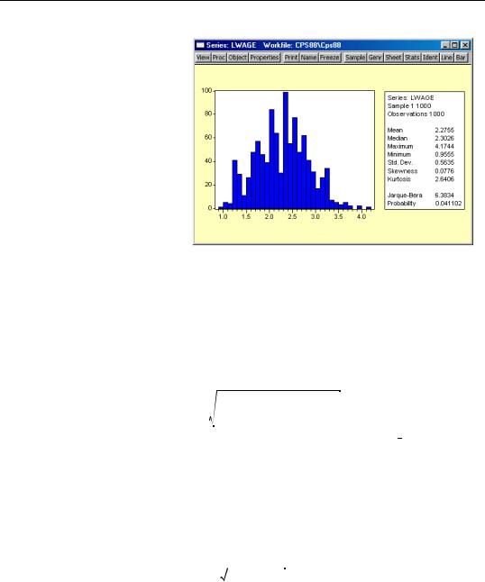
Histogram and Stats
This view displays the frequency distribution of your series in a histogram. The histogram divides the series range (the distance between
the maximum and minimum values) into a number of equal length intervals or bins and displays a count of the number of observations that fall into each bin.
Descriptive Statistics—311
A complement of standard descriptive statistics are displayed along with the histogram. All of the statistics are calculated using the observations in the current sample.
•Mean is the average value of the series, obtained by adding up the series and dividing by the number of observations.
•Median is the middle
value (or average of the two middle values) of the series when the values are ordered from the smallest to the largest. The median is a robust measure of the center of the distribution that is less sensitive to outliers than the mean.
•Max and Min are the maximum and minimum values of the series in the current sample.
•Std. Dev. (standard deviation) is a measure of dispersion or spread in the series. The standard deviation is given by:
s = |
|
N |
|
2 |
⁄ ( N − 1 ) |
|
|
|
|
||||
|
Σ ( yi − y) |
(11.1) |
||||
i = 1
where N is the number of observations in the current sample and y is the mean of the series.
•Skewness is a measure of asymmetry of the distribution of the series around its mean. Skewness is computed as:
|
1 N |
|
yi − |
|
3 |
|
|
S = |
y |
(11.2) |
|||||
---- |
Σ |
------------- |
|||||
|
|
|
ˆ |
|
|
|
|
|
Ni = 1 |
|
σ |
|
|
|
|
ˆ |
|
where σ is an estimator for the standard deviation that is based on the biased esti- |
|
ˆ |
( N − 1 ) ⁄ N) . The skewness of a symmetric distri- |
mator for the variance ( σ = s |
|
bution, such as the normal distribution, is zero. Positive skewness means that the distribution has a long right tail and negative skewness implies that the distribution has a long left tail.

312—Chapter 11. Series
•Kurtosis measures the peakedness or flatness of the distribution of the series. Kurtosis is computed as
|
1 N |
|
yi |
− |
|
4 |
|
|
K = |
y |
(11.3) |
||||||
---- |
Σ |
------------- |
||||||
|
|
|
|
ˆ |
|
|
|
|
|
Ni = 1 |
|
|
σ |
|
|
|
|
where σˆ is again based on the biased estimator for the variance. The kurtosis of the normal distribution is 3. If the kurtosis exceeds 3, the distribution is peaked (leptokurtic) relative to the normal; if the kurtosis is less than 3, the distribution is flat (platykurtic) relative to the normal.
•Jarque-Bera is a test statistic for testing whether the series is normally distributed. The test statistic measures the difference of the skewness and kurtosis of the series with those from the normal distribution. The statistic is computed as:
Jarque-Bera = |
N − k |
2 |
+ |
(K − 3)2 |
(11.4) |
-------------6 S |
|
--------------------4 - |
where S is the skewness, K is the kurtosis, and k represents the number of estimated coefficients used to create the series.
Under the null hypothesis of a normal distribution, the Jarque-Bera statistic is distributed as χ2 with 2 degrees of freedom. The reported Probability is the probability that a Jarque-Bera statistic exceeds (in absolute value) the observed value under the null hypothesis—a small probability value leads to the rejection of the null hypothesis of a normal distribution. For the LWAGE series displayed above, we reject the hypothesis of normal distribution at the 5% level but not at the 1% significance level.
Stats Table
Displays slightly more information than the Histogram/Stats view, with the numbers displayed in tabular form.
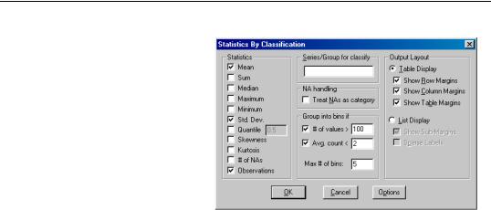
Stats by Classification
This view allows you to compute the descriptive statistics of a series for various subgroups of your sample. If you select View/Descriptive Statistics/Stats by Classification… a Statistics by Classification dialog box appears:
Descriptive Statistics—313
The Statistics option at the left allows you to choose the statistic(s) you wish to compute.
In the Series/Group for Classify field enter series or group names that define your subgroups. You must type at least one name.
Descriptive statistics will be calculated for each unique value of the classification series unless binning is selected. You may type more than one series or group
name; separate each name by a space. The quantile statistic requires an additional argument (a number between 0 and 1) corresponding to the desired quantile value. Click on the Options button to choose between various methods of computing the quantiles. See “CDF-Survivor-Quantile” on page 391 for details.
By default, EViews excludes observations which have missing values for any of the classification series. To treat NA values as a valid subgroup, select the NA handling option.
The Layout option allows you to control the display of the statistics. Table layout arrays the statistics in cells of two-way tables. The list form displays the statistics in a single line for each classification group.
The Table and List options are only relevant if you use more than one series as a classifier.
The Sparse Labels option suppresses repeating labels in list mode to make the display less cluttered.
The Row Margins, Column Margins, and Table Margins instruct EViews to compute statistics for aggregates of your subgroups. For example, if you classify your sample on the basis of gender and age, EViews will compute the statistics for each gender/age combination. If you elect to compute the marginal statistics, EViews will also compute statistics corresponding to each gender, and each age subgroup.
A classification may result in a large number of distinct values with very small cell sizes. By default, EViews automatically groups observations into categories to maintain moderate cell sizes and numbers of categories. Group into Bins provides you with control over this process.
Setting the # of values option tells EViews to group data if the classifier series takes more than the specified number of distinct values.

314—Chapter 11. Series
The Avg. count option is used to bin the series if the average count for each distinct value of the classifier series is less than the specified number.
The Max # of bins specifies the maximum number of subgroups to bin the series. Note that this number only provides you with approximate control over the number of bins.
The default setting is to bin the series into 5 subgroups if either the series takes more than 100 distinct values or if the average count is less than 2. If you do not want to bin the series, unmark both options.
For example, consider the following stats by classification view in table form:
Descriptive Statistics for LWAGE
Categorized by values of MARRIED and UNION
Date: 10/15/97 Time: 01:11
Sample: 1 1000
Included observations: 1000
Mean |
|
|
|
Median |
|
|
|
Std. Dev. |
|
UNION |
|
Obs. |
0 |
1 |
All |
0 |
1.993829 |
2.387019 |
2.052972 |
|
1.906575 |
2.409131 |
2.014903 |
|
0.574636 |
0.395838 |
0.568689 |
|
305 |
54 |
359 |
MARRIED 1 |
2.368924 |
2.492371 |
2.400123 |
|
2.327278 |
2.525729 |
2.397895 |
|
0.557405 |
0.380441 |
0.520910 |
|
479 |
162 |
641 |
All |
2.223001 |
2.466033 |
2.275496 |
|
2.197225 |
2.500525 |
2.302585 |
|
0.592757 |
0.386134 |
0.563464 |
|
784 |
216 |
1000 |
|
|
|
|
The header indicates that the table cells are categorized by two series MARRIED and UNION. These two series are dummy variables that take only two values. No binning is performed; if the series were binned, intervals rather than a number would be displayed in the margins.
The upper left cell of the table indicates the reported statistics in each cell; in this case, the median and the number of observations are reported in each cell. The row and column labeled All correspond to the Row Margin and Column Margin options described above.
Here is the same view in list form with sparse labels: