


120—Chapter 5. Basic Data Handling
Overriding Default Conversion Methods
If you use copy-and-paste to copy one or more series between two workfiles, EViews will copy the series to the destination page, using the default frequency conversion settings present in the series to perform the conversion.
If, when pasting the series into the destination, you use Paste Special... in place of Paste, EViews will display a dialog offering you the opportunity to override the default frequency conversion settings.
You need not concern yourself with most of the settings in this dialog at the moment; the dialog is discussed in greater detail in “Frequency conversion links” on page 198.
We note, however, that the dialog offers us the opportunity to change both the name of the pasted YQ series, and the frequency conversion method.
The “*” wildcard in the Pattern field is used to indicate that we will
use the original name (wildcards are most useful when pasting multiple series). We may edit the field to provide a name or alternate wildcard pattern. For example, changing this setting to “*A” would copy the YQ series as YQA in the destination workfile.
Additionally, we note that the dialog allows us to use the frequency conversion method Specified in series or to select alternative methods.
If, instead of copy-and-paste, you are using either the copy or fetch command and you provide an option to set the conversion method, then EViews will use this method for all of the series listed in the command (see copy (p. 249) and fetch (p. 291) in the Command and Programming Reference for details).
Importing ASCII Text Files
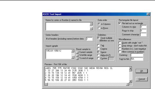
To import an ASCII text file, click on Proc/Import/Read Text-Lotus-Excel... from the main menu or the workfile toolbar, and select the file in the File Open dialog. The ASCII Text Import dialog will be displayed.
Importing ASCII Text Files—121
You may notice that the dialog is more complicated than the corresponding spreadsheet dialog. Since there is no standard format for ASCII text files, we need to provide a variety of options to handle various types of files.
Note that the
preview window at the bottom of the dialog shows you the first 16K of your file. You can use this information to set the various formatting options in the dialog.
You must provide the following information:
•Names for series or Number of series if names in file. If the file does not contain series names, or if you do not want to use the names in the file, list the names of the series in the order they appear in the file, separated by spaces.
If the names of the series are located in the file before the start of the data, you can tell EViews to use these names by entering a number representing the number of series to be read.
If possible, you should avoid using parentheses and mathematical symbols such as “*”, “+”, “-”, “/”, “^” in the series names in the file. If EViews tries to read the names from the file and encounters an invalid name, it will try to rename the series to a valid name by replacing invalid characters with underscores and numbers. For example, if the series is named “X(-3)” in the file, EViews will rename this series to “X__3_01”. If “X__3_01” is already a series name, then EViews will name the series “X__3_02”, and so forth.
If EViews cannot name your series, say, because the name is a reserved name, or because the name is used by an object that is not a series, the series will be named “SER01”, “SER02”, etc.

122—Chapter 5. Basic Data Handling
You should be very careful in naming your series and listing the names in the dialog. If the name in the list or in the file is the same as an existing series name in the workfile, the data in the existing series will be overwritten.
•Data order. You need to specify how the data are organized in your file. If your data are ordered by observation so that each series is in a column, select in Columns. If your data are ordered by series so that all the data for the first series are in one row followed by all the data for the second series, and so on, select, in Rows.
•Import sample. You should specify the sample in which to place the data from the file. EViews fills out the dialog with the current workfile sample, but you can edit the sample string or use the sample reset buttons to change the input sample. The input sample only sets the sample for the import procedure, it does not alter the workfile sample.
EViews fills all of the observations in the current sample using the data in the input file. There are a couple of rules to keep in mind:
1.EViews assigns values to all observations in the input sample. Observations outside of the input sample will not be changed.
2.If there are too few values in the input file, EViews will assign NAs to the extra observations in the sample.
3.Once all of the data for the sample have been read, the remainder of the input file will be ignored.
In addition to the above information, you can use the following options to further control the way EViews reads in ASCII data.
EViews scans the first few lines of the source file and sets the default formatting options in the dialog based on what it finds. However, these settings are based on a limited number of lines and may not be appropriate. You may find that you need to reset these options.
Delimiters
Delimiters are the characters that your file uses to separate observations. You can specify multiple delimiters by selecting the appropriate entries. Tab, Comma, and Space are selfexplanatory. The Alpha option treats any of the 26 characters from the alphabet as a delimiter.
For delimiters not listed in the option list, you can select the Custom option and specify the symbols you wish to treat as delimiters. For example, you can treat the slash “/” as a delimiter by selecting Custom and entering the character in the edit box. If you enter more than one character, each character will be treated as a delimiter. For example, if you enter double slash “//” in the Custom field, then the single slash “/” will be treated as a delim-
Importing ASCII Text Files—123
iter, instead of the double slash “//”. The double slash will be interpreted as two delimiters.
EViews provides you with the option of treating multiple delimiter characters as a single delimiter. For example, if “,” is a delimiter and the option Treat multiple delimiters as one is selected, EViews will interpret “,,” as a single delimiter. If the option is turned off, EViews will view this string as two delimiters surrounding a missing value.
Rectangular File Layout Options
To treat the ASCII file as a rectangular file, select the File laid out as rectangle option in the upper right-hand portion of the dialog. If the file is rectangular, EViews reads the file as a set of lines, with each new line denoting a new observation or a new series, depending on whether you are reading by column or by row. If you turn off the rectangular option, EViews treats the whole file as one long string separated by delimiters and carriage returns.
Knowing that a file is rectangular simplifies ASCII reading since EViews knows how many values to expect on a given line. For files that are not rectangular, you will need to be precise about the number of series or observations that are in your file. For example, suppose that you have a non-rectangular file that is ordered in columns and you tell EViews that there are four series in the file. EViews will ignore new lines and will read a new observation after reading every four values.
If the file is rectangular, you can tell EViews to skip columns and/or rows.
For example, if you have a rectangular file and you type 3 in the Rows to skip field, EViews will skip the first three rows of the data file. Note that you can only skip the first few rows or columns; you cannot skip rows or columns in the middle of the file.
Series Headers
This option tells EViews how many “cells” to offset as series name headers before reading the data in the file. The way that cell offsets are counted differs depending on whether the file is in rectangular form or not.
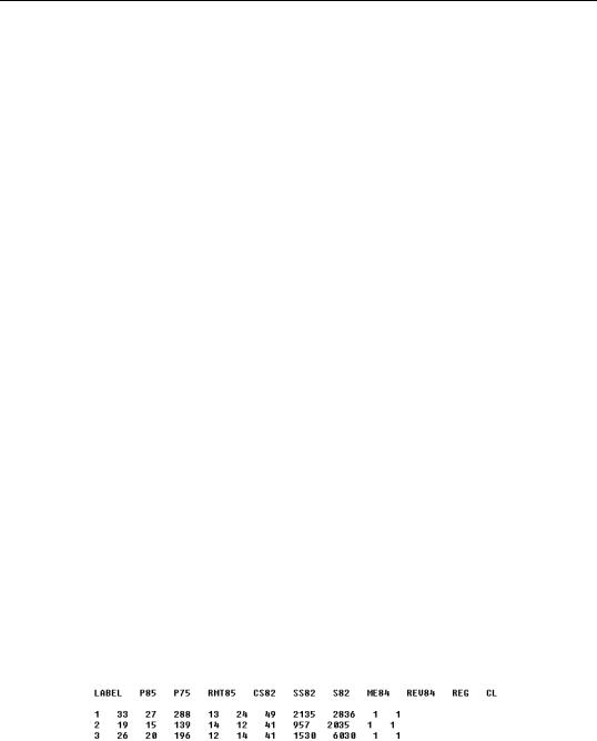
For files in rectangular form, the offsets are given by rows (for data in columns) or by columns (for data in rows). For example, suppose your data file looks as follows:
There is a one line (row) gap between the series name line and the data for the first observation. In this case, you should set the series header offset as 2, one for the series name line and one for the gap. If there were no gap, then the correct offset would instead be 1.
124—Chapter 5. Basic Data Handling
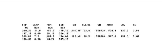
For files not in rectangular form, the offsets are given by the number of cells separated by the delimiters. For example, suppose you have a data file that looks as follows:
The data are ordered in columns, but each observation is recorded in two lines, the first line for the first 10 series and the second line for the remaining 4 series.
It is instructive to examine what happens if you incorrectly read this file as a rectangular file with 14 series and a header offset of 2. EViews will look for the series names in the first line, will skip the second line, and will begin reading data starting with the third line, treating each line as one observation. The first 10 series names will be read correctly, but since EViews will be unable to find the remaining four names on the first line, the remaining series will be named SER01–SER04. The data will also be read incorrectly. For example, the first four observations for the series GR will be 215.9800, NA, 180.4800, and NA, since EViews treats each line as a new observation.
To read this data file properly, you should turn off the rectangle file option and set the header offset to 1. Then EViews will read, from left to right, the first 14 values that are separated by a delimiter or carriage return and take them as series names. This corresponds to the header offset of 1, where EViews looks to the number of series (in the upper left edit box) to determine how many cells to read per header offset. The next 14 observations are the first observations of the 14 series, and so on.
Miscellaneous Options
•Quote with single ‘ not “. The default behavior in EViews is to treat anything inside a pair of matching double quotes as one string, unless it is a number. This option treats anything inside a pair of matching single quotes as one string, instead of the double quotes. Since EViews does not support strings, the occurrence of a pair of matching double quotes will be treated as missing, unless the text inside the pair of double quotes may be interpreted as a number.
•Drop strings—don’t make NA. Any input into a numeric series that is not a number or delimiter will, by default, be treated as a missing observation. For example, “10b” and “90:4” will both be treated as missing values (unless Alphabetic characters or “:” are treated as delimiters). The Drop strings option will skip these strings instead of treating them as NAs.
If you choose this option, the series names, which are strings, will also be skipped so that your series will be named using the EViews default names: “SER01”,

Importing ASCII Text Files—125
“SER02”, and so on. If you wish to name your series, you should list the series names in the dialog.
Note that strings that are specified as missing observations in the Text for NA edit box will not be skipped and will be properly indicated as missing.
•Numbers in ( ) are negative. By default, EViews treats parentheses as strings. However, if you choose this option, numbers in parentheses will be treated as negative numbers and will be read accordingly.
•Allow commas in numbers. By default, commas are treated as strings unless you specify them as a delimiter. For example, “1,000” will be read as either NA (unless you choose the drop string option, in which case it will be skipped) or as two observations, 1 and 0 (if the comma is a delimiter). However, if you choose to Allow commas in numbers, “1,000” will be read as the number 1000.
•Currency. This option allows you to specify a symbol for currency. For example, the default behavior treats “$10”’ as a string (which will either be NA or skipped) unless you specify “$” as a delimiter. If you enter “$” in the Currency option field, then “$10” will be read as the number 10.
The currency symbol can appear either at the beginning or end of a number but not in the middle. If you type more than one symbol in the field, each symbol will be treated as a currency code. Note that currency symbols are case sensitive. For example, if the Japanese yen is denoted by the “Y” prefix, you should enter “Y”, not “y”.
•Text for NA. This option allows you to specify a code for missing observations. The default is NA. You can use this option to read data files that use special values to indicate missing values, e.g., “.”, or “-99”.
You can specify only one code for missing observations. The entire Text for NA string will be treated as the missing value code.
Examples
In these examples, we demonstrate the ASCII import options using example data files downloaded from the Internet. The first example file looks as follows:
This is a cross-section data set, with seven series ordered in columns, each separated by a single space. Note that the B series takes string values, which will be replaced by NAs. If we type 7 series in the number of series field and use the default setting, EViews will correctly read the data.
126—Chapter 5. Basic Data Handling
By default, EViews checks the Treat multiple delimiters as one option even though the series are delimited by a single space. If you do not check this option, the last series BB will not be read. EViews will create a series named “SER01” and all data will be incorrectly imported. This strange behavior is caused by an extra space in the very first column of the data file, before the 1st and 3rd observations of the X series. EViews treats the very first space as a delimiter and looks for the first series data before the first extra space, which is missing. Therefore the first series is named SER01 with data NA, 10, NA, 12 and all other series are incorrectly imported.
To handle this case, EViews automatically ignores the delimiter before the first column data if you choose both the Treat multiple delimiters as one and the File laid out as rectangle options.
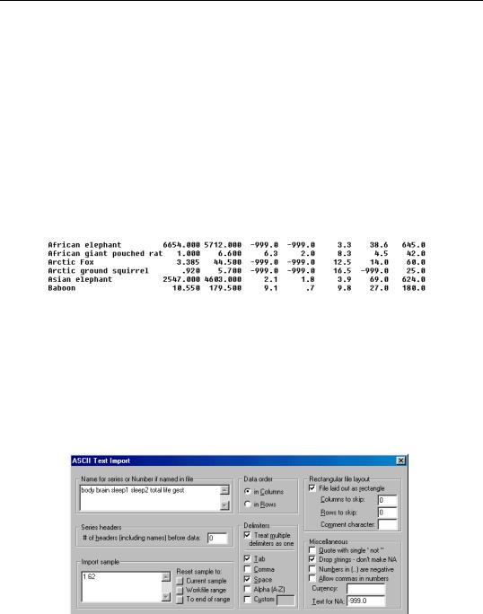
The top of the second example file looks like:
This is a cross-section data set, ordered in columns, with missing values coded as “-999.0”. There are eight series, each separated by spaces. The first series is the ID name in strings.
If we use the EViews defaults, there will be problems reading this file. The spaces in the ID description will generate spurious NA values in each row, breaking the rectangular format of the file. For example, the first name will generate two NAs, since “African” is treated as one string, and “elephant” as another string.
You will need to use the Drop strings option to skip all of the strings in your data so that you don’t generate NAs. Fill out the ASCII dialog as follows:
Note the following:
Importing ASCII Text Files—127
•Since we skip the first string series, we list only the remaining seven series names.
•There are no header lines in the file, so we set the offset to 0.
•If you are not sure whether the delimiter is a space or tab, mark both options. You should treat multiple delimiters as one.
•Text for NA should be entered exactly as it appears in the file. For this example, you should enter “–999.0”, not “–999”.
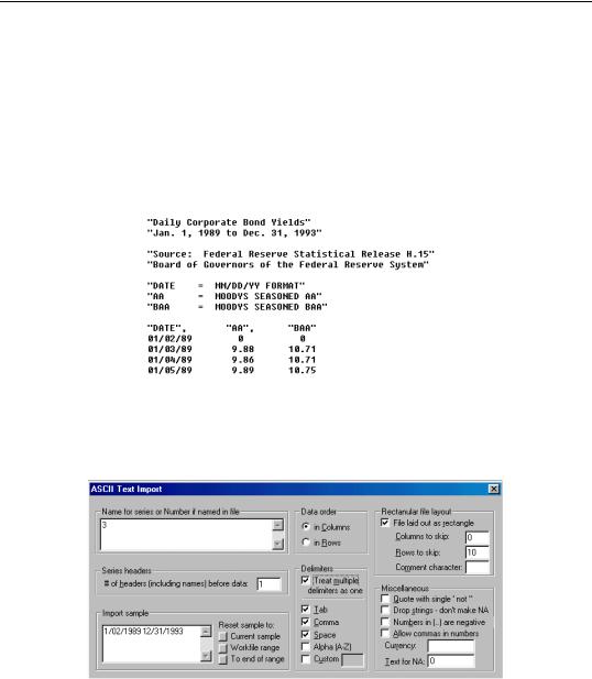
The third example is a daily data file that looks as follows:
This file has 10 lines of data description, line 11 is the series name header, and the data begin in line 12. The data are ordered in columns in rectangular form with missing values coded as a “0”. To read these data, you can instruct EViews to skip the first 10 rows of the rectangular file, and read three series with the names in the file, and NAs coded as “0”.
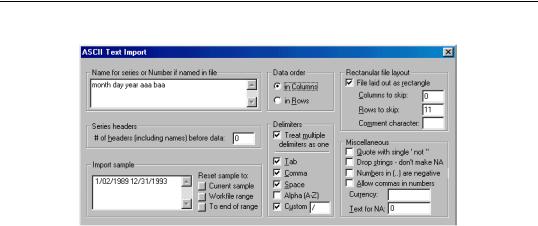
The only problem with this method is that the DATE series will be filled with NAs since EViews treats the entry as a string (because of the “/” in the date entry). You can avoid this problem by identifying the slash as a delimiter using the Custom edit box. The first column will now be read as three distinct series since the two slashes are treated as delimiters. Therefore, we modify the option settings as follows:
128—Chapter 5. Basic Data Handling
Note the changes to the dialog entries:
•We now list five series names. We cannot use the file header since the line only contains three names.
•We skip 11 rows with no header offset since we want to skip the name header line.
•We specify the slash “/” as an additional delimiter in the Custom option field.
The month, day, and year will be read as separate series and can be used as a quick check of whether the data have been read correctly.