274—Chapter 10. EViews Databases

Database Auto-Series

We have described how to fetch series into a workfile. There is an alternative way of working with databases which allows you to make direct use of the series contained in a database without first copying the series. The advantage of this approach is that you need not go through the process of importing the data every time the database is revised. This approach follows the model of auto-series in EViews as described in “Auto-series” beginning on page 141.

There are many places in EViews where you can use a series expression, such as log(X), instead of a simple series name, and EViews will automatically create a temporary autoseries for use in the procedure. This functionality has been extended so that you can now directly refer to a series in a database using the syntax:

db_name::object_name

where db_name is the shorthand associated with the database. If you omit the database name and simply prefix the object name with a double colon like this:

::object_name

EViews will look for the object in the default database.

A simple example is to generate a new series:

series lgdp = log(macro_db::gdp)

EViews will fetch the series named GDP from the database with the shorthand MACRO_DB, and put the log of GDP in a new series named LGDP in the workfile. It then deletes the series GDP from memory, unless it is in use by another object. Note that the generated series LGDP only contains data for observations within the current workfile sample.

You can also use auto-series in a regression. For example:

equation eq1.ls log(db1::y) c log(db2::x)

This will fetch the series named Y and X from the databases named DB1 and DB2, perform any necessary frequency conversions and end point truncation so that they are suitable for use in the current workfile, take the log of each of the series, then run the requested regression. Y and X are then deleted from memory unless they are otherwise in use.

The auto-series feature can be further extended to include automatic searching of databases according to rules set in the database registry (see “The Database Registry” on page 275). Using the database registry you can specify a list of databases to search whenever a series you request cannot be found in the workfile. With this feature enabled, the series command:

The Database Registry—275

series lgdp = log(gdp)

looks in the workfile for a series named GDP. If it is not found, EViews will search through the list of databases one by one until a series called GDP is found. When found, the series will be fetched into EViews so that the expression can be evaluated. Similarly, the regression:

equation logyeq.ls log(y) c log(x)

will fetch Y and X from the list of databases in the registry if they are not found in the workfile. Note that the regression output will label all variables with the database name from which they were imported.

In general, using auto-series directly from the database has the advantage that the data will be completely up to date. If the series in the database are revised, you do not need to repeat the step of importing the data into the workfile. You can simply reestimate the equation or model, and EViews will automatically retrieve new copies of any data which are required.

There is one complication to this discussion which results from the rules which regulate the updating and deletion of auto-series in general. If there is an existing copy of an autoseries already in use in EViews, a second use of the same expression will not cause the expression to be reevaluated (in this case reloaded from the database); it will simply make use of the existing copy. If the data in the database have changed since the last time the auto-series was loaded, the new expression will use the old data.

One implication of this behavior is that a copy of a series from a database can persist for any length of time if it is stored as a member in a group. For example, if you type:

show db1::y db2::x

this will create an untitled group in the workfile containing the expressions db1::y and db2::x. If the group window is left open and the data in the database are modified (for example by a store or a copy command), the group and its window will not update automatically. Furthermore, if the regression:

equation logyeq.ls log(db1::y) c log(db2::x)

is run again, this will use the copies of the series contained in the untitled group; it will not refetch the series from the database.

The Database Registry

The database registry is a file on disk that manages a variety of options which control database operations. It gives you the ability to assign short alias names that can be used in

276—Chapter 10. EViews Databases

place of complete database paths, and also allows you to configure the automatic searching features of EViews.

Options/Database Registry… from the main menu brings up the Database Registry dialog allowing you to view and edit the database registry:

The box labeled Registry Entries lists the databases that have been registered with EViews. The first time you bring up the dialog, the box will usually be empty. If you click on the Add new entry button, a Database Registry Entry dialog appears.

There are three things you must specify in the dialog: the full name (including path) of the database, the alias which you would like to associate with the database, and the option for whether you wish to include the database in automatic searches.

The full name and path of the database should be entered in the top edit field. Alternatively, click the Browse button to select your database interactively.

The next piece of information you must provide is a database alias: a short name that you can use in place of the full database path in EViews commands. The database alias will

also be used by EViews to label database auto-series. For example, suppose you have a database named DRIBASIC located in the subdirectory C:\EVIEWS\DATA. The following regression command is legal but awkward:

equation eq1.ls c:\eviews\data\dribasic::gdp c c:\eviews\data\dribasic::gdp(-1)

Long database names such as these also cause output labels to truncate, making it difficult to see which series were used in a procedure.

Querying the Database—277

By assigning full database path and name the alias DRI, we may employ the more readable command:

equation eq1.ls dri::gdp c dri::gdp(-1)

and the regression output will be labeled with the shorter names. To minimize the possibility of truncation, we recommend the use of short alias names if you intend to make use of database auto-series.

Finally, you should tell EViews if you want to include the database in automatic database searches by checking the Include in auto search checkbox. Click on OK to add your entry to the list

Any registry entry may be edited, deleted, switched on or off for searching, or moved to the top of the search order by highlighting the entry in the list and clicking the appropriate button to the right of the list box.

The remainder of the Database Registry dialog allows you to set options for automatic database searching. The Auto-search checkbox is used to control EViews behavior when you enter a command involving a series name which cannot be found in the current workfile. If this checkbox is selected, EViews will automatically search all databases that are registered for searching, before returning an error. If a series with the unrecognized name is found in any of the databases, EViews will create a database auto-series and continue with the procedure.

The last section of the dialog, Default Database in Search Order, lets you specify how the default database is treated in automatic database searches. Normally, when performing an automatic search, EViews will search through the databases contained in the Registry Entries window in the order that they are listed (provided that the Include in auto search box for that entry has been checked). These options allow you to assign a special role to the default database when performing a search.

•Include at start of search order—means that the current default database will be searched first, before searching the listed databases.

•Include at end of search order—means that the current default database will be searched last, after searching the listed databases.

•Do not include in search—means that the current default database will not be searched unless it is already one of the listed databases.

Querying the Database

A great deal of the power of the database comes from its extensive query capabilities. These capabilities make it easy to locate a particular object, and to perform operations on a set of objects which share similar properties.

278—Chapter 10. EViews Databases

The query capabilities of the database can only be used interactively from the database window. There are two ways of performing a query on the database: the easy mode and the advanced mode. Both methods are really just different ways of building up a text query to the database. The easy mode provides a simpler interface for performing the most common types of queries. The advanced mode offers more flexibility at the cost of increased complexity.

Easy Queries

To perform an easy query, first open the database, then click on the EasyQuery button in the toolbar at the top of the database window. The Easy Query dialog will appear containing two text fields and a number of check boxes:

There are two main sections to this dialog: Select and Where. The Select section determines which fields to display for each object that meets the query condition. The Where section allows you to specify conditions that must be met for an object to be returned from the query. An Easy Query allows you to set conditions on the object name, object description, and/or object type.

The two edit fields (name and description) and the set of check boxes (object type) in the Where section provide three filters of objects that are returned from the query to the database. The filters are applied in sequence (using a logi-

cal ‘and’ operation) so that objects in the database must meet all of the criteria selected in order to appear in the results window of the query.

The name and description fields are each used to specify a pattern expression that the object must meet in order to satisfy the query. The simplest possible pattern expression consists of a single pattern. A pattern can either be a simple word consisting of alphanumeric characters, or a pattern made up of a combination of alphanumeric characters and the wildcard symbols “?” and “*”, where “?” means to match any one character and “*” means to match zero or more characters. For example:

pr?d*ction

would successfully match the words production, prediction, and predilection. Frequently used patterns include “s*” for words beginning in “S”, “*s” for words ending in “S”, and “*s*” for words containing “S”. Upper or lower case is not significant when searching for matches.

280—Chapter 10. EViews Databases

Advanced Queries

Advanced queries allow considerably more control over both the filtering and the results which are displayed from a query. Because of this flexibility, advanced queries require some understanding of the structure of an EViews database to be used effectively.

Each object in an EViews database is described by a set of fields. Each field is identified by a name. The current list of fields includes:

An advanced query allows you to examine the contents of any of these fields, and to select objects from the database by placing conditions on these fields. An advanced query can be performed by opening the database window, then clicking on the button marked Query in the toolbar at the top of the window. The Advanced Query dialog is displayed.

Querying the Database—281

The first edit field labeled Select: is used to specify a list of all the fields that you would like displayed in the query results. Input into this text box consists of a series of field names separated by commas. Note that the name and type fields are always fetched automatically.

The ordering of display of the results of a query is determined by the Order By edit field. Any field name can be entered into this box, though some fields are likely to be more useful than others. The description field, for example, does not provide a useful ordering of the objects. The Order By field can be useful for

grouping together objects with the same value of a particular field. For example, ordering by type is an effective way to group together the results so that objects of the same type are placed together in the database window. The Ascending and Descending buttons can be used to reverse the ordering of the objects. For example, to see objects listed from those most recently written in the database to those least recently written, one could simply sort by the field last_write in Descending order.

The Where edit field is the most complicated part of the query. Input consists of a logical expression built up from conditions on the fields of the database. The simplest expression is an operator applied to a single field of the database. For example, to search for all series which are of monthly or higher frequencies (where higher frequency means containing more observations per time interval), the appropriate expression is:

freq >= monthly

Field expressions can also be combined with the logical operators and, or and not with precedence following the same rules as those described above in the section on easy queries. For example, to query for all series of monthly or higher frequencies which begin before 1950, we could enter the expression:

freq >= monthly and start < 1950

Each field has its own rules as to the operators and constants which can be used with the field.

Name

The name field supports the operators “<“, “<=”, “>”, “>=”, “=”, and “<>” to perform typical comparisons on the name string using alphabetical ordering. For example,

282—Chapter 10. EViews Databases

name >= c and name < m

will match all objects with names beginning with letters from C to L. The name field also supports the operator “matches”. This is the operator which is used for filtering the name field in the easy query and is documented extensively in the previous section. Note that if matches is used with an expression involving more than one word, the expression must be contained in quotation marks. For example,

name matches "x* or y*" and freq = quarterly

is a valid query, while

name matches x* or y* and freq = quarterly

is a syntax error because the part of the expression that is related to the matches operator is ambiguous.

Type

The type field can be compared to the following object types in EViews using the “=” operator: sample, equation, graph, table, text, program, model, system, var, pool, sspace, matrix, group, sym, matrix, vector, coef, series. Relational operators are defined for the type field, although there is no particular logic to the ordering. The ordering can be used, however, to group together objects of similar types in the Order By field.

Freq

The frequency field has one of the following values:

Any word beginning with the letter above is taken to denote that particular frequency, so that monthly can either be written as “m” or “monthly”. Ordering over frequencies is defined so that a frequency with more observations per time interval is considered “greater” than a series with fewer observations per time interval. The operators “<”, “>”, “<=”, “>=”, “=”, “<>” are all defined according to these rules. For example,

284—Chapter 10. EViews Databases

last_write >= mm/dd/yyyy

A day constant always refers to twelve o’clock midnight at the beginning of that day. There is no way to specify a particular time during the day.

Description, Source, Units, Remarks, History, Display_name

These fields contain the label information associated with each object (which can be edited using the Label view of the object in the workfile). Only one operator is available on these fields, the matches operator, which behaves exactly the same as the description field in the section on easy queries.

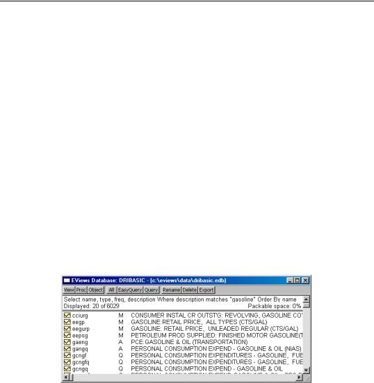
Query Examples

Suppose you are looking for data related to gasoline consumption and gasoline prices in the database named DRIBASIC. First open the database: click File/Open, select Files of type: Database .edb and locate the database. From the database window, click Query and fill in the Advanced Query dialog as follows:

Select: name, type, freq, description

Where: description matches gasoline

If there are any matches, the results are displayed in the database window similar to the following:

To view the contents of all fields of an item, double click on its name. EViews will open an Object Description window that looks as follows: