


Auto-series—141
There are alternative forms for the assignment statement. First, if the series does not exist, you must use either the series or the genr keyword, followed by the assignment expression. The two statements:
series y = exp(x)
genr y = exp(x)
are equivalent methods of generating the series Y. Once the series has been created, subsequent assignment statements do not require the series or the genr keyword:
smpl @all
series y = exp(x)
smpl 1950 1990 if y>300
y = y/2
This set of commands first sets the series to equal EXP(X) for all observations, then assigns the values Y/2 for the subset of observations from 1950 to 1990 if Y>300.
Auto-series
Another important method of working with expressions is to use an expression in place of a series. EViews’ powerful tools for expression handling allow you to substitute expressions virtually any place you would use a series—as a series object, as a group element, in equation specifications and estimation, and in models.
We term expressions that are used in place of series as auto-series, since the transformations in the expressions are automatically calculated without an explicit assignment statement.
Auto-series are most useful when you wish to see the behavior of an expression involving one ore more series, but do not want to keep the transformed series, or in cases where the underlying series data change frequently. Since the auto-series expressions are automatically recalculated whenever the underlying data change, they are never out-of-date.
See “Auto-Updating Series” on page 149 for a more advanced method of handling series and expressions.
Creating Auto-series
It is easy to create and use an auto-series—anywhere you might use a series name, simply enter an EViews expression. For example, suppose that you wish to plot the log of CP against time for the period 1953M01 to 1958M12. There are two ways in which you might plot these values.
One way to plot these values is to generate an ordinary series, as described earlier in “Basic Assignment” on page 138, and then to plot its values. To generate an ordinary series
142—Chapter 6. Working with Data
containing the log of CP, say with the name LOGCP, select Quick/Generate series... from the main menu, and enter,
logcp = log(cp)
or type the command,
series logcp = log(cp)
in the command window. EViews will evaluate the expression LOG(CP) for the current values of CP, and will place these values into the series LOGCP. To view a line graph view of the series, open the series LOGCP and select View/Graph/Line.
Note that the values of the ordinary series LOGCP will not change when CP is altered. If you wish to update the values in LOGCP to reflect subsequent changes in CP, you will need to issue another series or genr assignment statement.
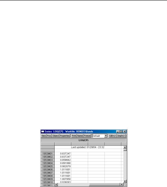
Alternatively, you may create and use an auto-series by clicking on the Show button on the toolbar, or selecting Quick/Show… and entering the command,
log(cp)
or by typing
show log(cp)
in the command window. EViews will open a series window in spreadsheet view:
Note that in place of an actual series name, EViews substitutes the expression used to create the auto-series.
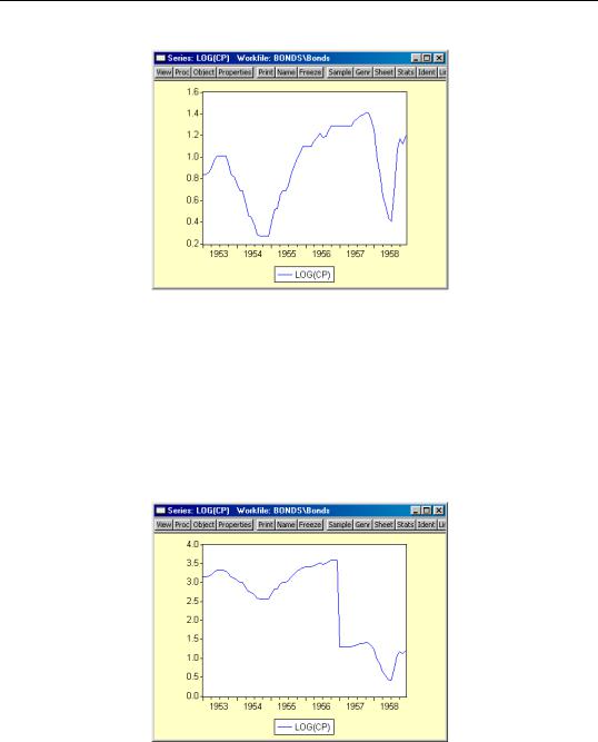
An auto-series may be treated as a standard series window so all of the series views and procedures are immediately available. To display a time series graph of the LOG(CP) autoseries, simply select View/Graph/Line from the series window toolbar:
Auto-series—143
All of the standard series views and procedures are also accessible from the menus.
Note that if the data in the CP series are altered, the auto-series will reflect these changes. Suppose, for example, that we take the first four years of the CP series, and multiply theme by a factor of 10:
smpl 1953m01 1956m12
cp = cp*10
smpl 1953m01 1958m12
The auto-series graph will automatically change to reflect the new data:
In contrast, the values of the ordinary series LOGCP are not affected by the changes in the CP data.
144—Chapter 6. Working with Data
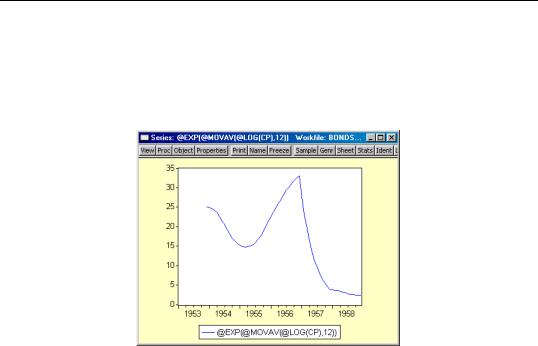
Similarly, you may use an auto-series to compute a 12-period, backward-looking, geometric moving average of the updated CP data. The command:
show @exp(@movav(@log(cp),12))
will display the auto-series containing the geometric moving average:
Naming an Auto-series
The auto-series is deleted from your computer memory when you close the series window containing the auto-series. For more permanent expression handling, you may convert the auto-series into an auto-updating series that will be kept in the workfile, by assigning a name to the auto-series.
Simply click on the Name button on the series toolbar, or select Object/Name... from the main menu, and provide a name. EViews will create an auto-updating series with that name in the workfile, and will assign the auto-series expression as the formula used in updating the series. For additional details, see “Auto-Updating Series” on page 149.
Using Auto-series in Groups
One of the more useful ways of working with auto-series is to include them in a group. Simply create the group as usual, using an expression in place of a series name, as appropriate. For example, if you select Object/New Object.../Group, and enter:
cp @exp(@movav(@log(cp),12))
you will create a group containing two series: the ordinary series CP, and the auto-series representing the geometric moving average. We may then use the group object graphing routines to compare the original series with the smoothed series: