


78—Chapter 4. Object Basics
Other multiple item selections are not valid, and will either issue an error or will simply not respond when you double click.
When you open an object, EViews will display the current view. In general, the current view of an object is the view that was displayed the last time the object was opened (if an object has never been opened, EViews will use a default view). The exception to this general rule is for those views that require significant computational time. In this latter case, the current view will revert to the default.
Showing Objects
An alternative method of selecting and opening objects is to “show” the item. Click on the Show button on the toolbar, or select Quick/Show… from the menu and type in the object name or names.
Showing an object works exactly as if you first selected the object or objects, and then opened your selection. If you enter a single object name in the dialog box, EViews will open the object as if you double clicked on the object name. If you enter multiple names, EViews will always open a single window to display results, creating a new object if necessary.
The Show button can also be used to display functions of series, also known as autoseries. All of the rules for auto-series that are outlined in “Database Auto-Series” on page 274, will apply.
The Object Window
We have been using the term object window somewhat loosely in the previous discussion of the process of creating and opening objects. Object windows are the windows that are displayed when you open an object or object container. An object’s window will contain either a view of the object, or the results of an object procedure.
One of the more important features of EViews is that you can display object windows for a number of items at the same time. Managing these object windows is similar to the task of managing pieces of paper on your desk.
Components of the Object Window
Let’s look again at a typical object window:
The Object Window—79
Here, we see the equation window for OLS_RESULTS. First, notice that this is a standard window which can be closed, resized, minimized, maximized, and scrolled both vertically and horizontally. As in other Windows applications, you can make an object window active by clicking once on the titlebar, or anywhere in its window. Making an object window active is equivalent to saying that you want to work with that object. Active windows may be identified by the darkened titlebar.
Second, note that the titlebar of the object window identifies the object type, name, and object container (in this case, the BONDS workfile or the OLS_RESULTS equation). If the object is itself an object container, the container information is replaced by directory information.
Lastly, at the top of the window there is a toolbar containing a number of buttons that provide easy access to frequently used menu items. These toolbars will vary across objects— the series object will have a different toolbar from an equation or a group or a VAR object.
There are several buttons that are found on all object toolbars:
•The View button lets you change the view that is displayed in the object window. The available choices will differ, depending upon the object type.
•The Proc button provides access to a menu of procedures that are available for the object.
•The Object button lets you manage your objects. You can store the object on disk, name, delete, copy, or print the object.
•The Print button lets you print the current view of the object (the window contents).
80—Chapter 4. Object Basics
•The Name button allows you to name or rename the object.
•The Freeze button creates a new object graph, table, or text object out of the current view.
Menus and the Object Toolbar
As we have seen, the toolbar provides a shortcut to frequently accessed menu commands. There are a couple of subtle, but important, points associated with this relationship that deserve special emphasis:
•Since the toolbar simply provides a shortcut to menu items, you can always find the toolbar commands in the menus.
•This fact turns out to be quite useful if your window is not large enough to display all of the buttons on the toolbar. You can either enlarge the window so that all of the buttons are displayed, or you can access the command directly from the menu.
•The toolbar and menu both change with the object type. In particular, the contents of the View menu and the Proc menu will always change to reflect the type of object (series, equation, group, etc.) that is active.
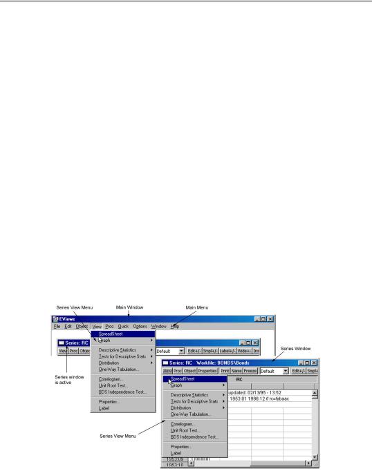
The toolbars and menus differ across objects. For example, the View and Proc drop-down menus differ for every object type. When the active window is displaying a series window, the menus provide access to series views and series procedures. Alternatively, when the active window is a group window, clicking on View or Proc in the main menu provides access to the different set of items associated with group objects.
The figure above illustrates the relationship between the View toolbar button and the View menu when the series window is the active window. In the left side of the illustration, we

Working with Objects—81
see a portion of the EViews main window, as it appears, after you click on View in the main menu (note that the RC series window is the active window). On the right, we see a depiction of the series window as it appears after you click on the View button in the series toolbar. Since the two operations are identical, the two drop-down menus are identical.
In contrast to the View and Proc menus, the Object menu does not, in general, vary across objects. An exception occurs, however, when an object container window (a workfile or database window) is active. In this case, clicking on Object in the toolbar, or selecting Object from the menu provides access to menu items for manipulating the objects in the container.
Working with Objects
Naming Objects
Objects may be named or unnamed. When you give an object a name, the name will appear in the directory of the workfile, and the object will be saved as part of the workfile when the workfile is saved.
You must name an object if you wish to keep its results. If you do not name an object, it will be called “UNTITLED”. Unnamed objects are not saved with the workfile, so they are deleted when the workfile is closed and removed from memory.
To rename an object, first open the object window by double clicking on its icon, or by clicking on Show on the workfile toolbar, and entering the object name. Next, click on the Name button on the object window, and enter the name (up to 24 characters), and optionally, a display name to be used when labelling the object in tables and graphs. If no display name is provided, EViews will use the object name.
You can also rename an object from the workfile window by selecting Object/Rename Selected… and then specifying the new object name. This method saves you from first having to open the object.
The following names are reserved and cannot be used as object names: ABS, ACOS, AND, AR, ASIN, C, CON, CNORM, COEF, COS, D, DLOG, DNORM, ELSE, ENDIF, EXP, LOG, LOGIT, LPT1, LPT2, MA, NA, NOT, NRND, OR, PDL, RESID, RND, SAR, SIN, SMA, SQR, and THEN.
EViews accepts both capital and lower case letters in the names you give to your series and other objects, but does not distinguish between names based on case. Its messages to you will follow normal capitalization rules. For example, “SALES”, “sales”, and “sAles” are all the same object in EViews. For the sake of uniformity, we have written all examples of input using names in lower case, but you should feel free to use capital letters instead.
82—Chapter 4. Object Basics
Despite the fact that names are not case sensitive, when you enter text information in an object, such as a plot legend or label information, your capitalization will be preserved.
By default, EViews allows only one untitled object of a given type (one series, one equation, etc.). If you create a new untitled object of an existing type, you will be prompted to name the original object, and if you do not provide one, EViews will replace the original untitled object with the new object. The original object will not be saved. If you prefer, you can instruct EViews to retain all untitled objects during a session but you must still name the ones you want to save with the workfile. See “Window and Font Options” on page 937.
Labeling Objects
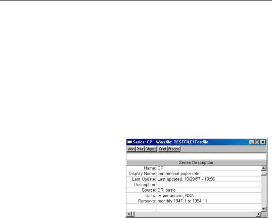
In addition to the display name described above, EViews objects have label fields where you can provide extended annotation and commentary. To view these fields, select View/ Label from the object window:
This is the label view of an unmodified object. By default, every time you modify the object, EViews automatically records the modification in a History field that will be appended at the bottom of the label view.
You can edit any of the fields, except the Last Update field. Simply click in the field cell that you
want to edit. All fields, except the Remarks and History fields, contain only one line. The Remarks and History fields can contain multiple lines. Press ENTER to add a new line to these two fields.
These annotated fields are most useful when you want to search for an object stored in an EViews database. Any text that is in the fields is searchable in an EViews database; see “Querying the Database” on page 277, for further discussion.
Copying Objects
There are two distinct methods of duplicating the information in an object: copying and freezing.
If you select Object/Copy from the menu, EViews will create a new untitled object containing an exact copy of the original object. By exact copy, we mean that the new object duplicates all the features of the original (except for the name). It contains all of the views and procedures of the original object and can be used in future analyses just like the original object.

Working with Objects—83
You may also copy an object from the workfile window. Simply highlight the object and click on Object/Copy Selected… or right mouse click and select Object/Copy..., then specify the destination name for the object.
We mention here that Copy is a very general and powerful operation with many additional features and uses. For example, you can copy objects across both workfiles and databases using wildcards and patterns. See “Copying Objects” on page 270, for details on these additional features.
Copy-and-Pasting Objects
The standard EViews copy command makes a copy of the object in the same workfile. When two workfiles are in memory at the same time, you may copy objects between them using copy-and-paste.
Highlight the objects you wish to copy in the source workfile. Then select Edit/Copy from the main menu.
Select the destination workfile by clicking on its titlebar. Then select either Edit/Paste or
Edit/Paste Special... from the main menu or simply Paste or Paste Special... following a right mouse click.
Edit/Paste will perform the default paste operation. For most objects, this involves simply copying over the entire object and its contents. In other cases, the default paste operation is more involved. For example, when copy-and-pasting series between source and destination workfiles that are of different frequency, frequency conversion will be performed, if possible, using the default series settings (see “Frequency Conversion” on page 115 for additional details). EViews will place named copies of all of the highlighted objects in the destination workfile, prompting you to replace existing objects with the same name.
If you elect to Paste Special..., EViews will open a dialog prompting you for any relevant paste options. For example, when pasting series, you may use the dialog to override the default series settings for frequency conversion, to perform special match merging by creating links (“Series Links” on page 177). In other settings, Paste Special... will simply prompt you to rename the objects in the destination workfile.
Freezing Objects
The second method of copying information from an object is to freeze a view of the object. If you click Object/Freeze Output or press the Freeze button on the object’s toolbar, a table or graph object is created that duplicates the current view of the original object.
Before you press Freeze, you are looking at a view of an object in the object window. Freezing the view makes a copy of the view and turns it into an independent object that will remain even if you delete the original object. A frozen view does not necessarily show what is currently in the original object, but rather shows a snapshot of the object at the

84—Chapter 4. Object Basics
moment you pushed the button. For example, if you freeze a spreadsheet view of a series, you will see a view of a new table object; if you freeze a graphical view of a series, you will see a view of a new graph object.
The primary feature of freezing an object is that the tables and graphs created by freezing may be edited for presentations or reports. Frozen views do not change when the workfile sample or data change.
Deleting Objects
To delete an object or objects from your workfile, select the object or objects in the workfile directory. When you have selected everything you want to delete, click Delete or Object/Delete Selected on the workfile toolbar. EViews will prompt you to make certain that you wish to delete the objects.
Printing Objects
To print the currently displayed view of an object, push the Print button on the object window toolbar. You can also choose File/Print or Object/Print on the main EViews menu bar.
EViews will open a Print dialog containing the default print settings for the type of output you are printing. Here, we see the dialog for printing text information; the dialog for printing from a graph will differ slightly.
The default settings for printer type, output redirection, orientation, and text size may be set in the Print Setup... dialog (see “Print Setup” on page 943) or they may be overridden in the current print dialog.
For example, the print commands normally send a view or procedure output to the current Windows printer. You may specify instead that the output should be saved in the workfile as a table or graph,
or spooled to an RTF or ASCII text file on disk. Simply click on Redirect, then select the output type from the list.
Storing Objects
EViews provides three ways to save your data on disk. You have already seen how to save entire workfiles, where all of the objects in the workfile are saved together in a single file

Working with Objects—85
with the .WF1 extension. You may also store individual objects in their own data bank files. They may then be fetched into other workfiles.
We will defer a full discussion of storing objects to data banks and databases until Chapter 10, “EViews Databases”, on page 261. For now, note that when you are working with an object, you can place it in a data bank or database file by clicking on the Object/ Store to DB… button on the object's toolbar or menu. EViews will prompt you for additional information.
You can store several objects, by selecting them in the workfile window and then pressing the Object/Store selected to DB… button on the workfile toolbar or menu.
Fetching Objects
You can fetch previously stored items from a data bank or database. One of the common methods of working with data is to create a workfile and then fetch previously stored data into the workfile as needed.
To fetch objects into a workfile, select Object/Fetch from DB… from the workfile menu or toolbar. You will see a dialog box prompting you for additional information for the fetch: objects to be fetched, directory and database location, as applicable.
See “Fetching Objects from the Database” on page 268, for details on the advanced features of the fetch procedure.
Updating Objects
Updating works like fetching objects, but requires that the objects be present in the workfile. To update objects in the workfile, select them from the workfile window, and click on Object/Update from DB… from the workfile menu or toolbar. The Fetch dialog will open, but with the objects to be fetched already filled in. Simply specify the directory and database location and click OK.
The selected objects will be replaced by their counterparts in the data bank or database.
See Chapter 10, “EViews Databases”, on page 261, for additional details on the process of updating objects from a database.
Copy-and-Paste of Object Information
You can copy the list of object information displayed in a workfile or database window to the Windows clipboard and paste the list to other program files such as word processing files or spreadsheet files. Simply highlight the objects in the workfile directory window, select Edit/Copy (or click anywhere in the highlighted area, with the right mouse button, and select Copy). Then move to the application (word processor or spreadsheet) where you want to paste the list, and select Edit/Paste.

86—Chapter 4. Object Basics
If only names are displayed in the window, EViews will copy a single line containing the highlighted names to the clipboard, with each name separated by a space. If the window contains additional information, either because View/Display Comments (Label+/–) has been chosen in a workfile window or a query has been carried out in a database window, each name will be placed in a separate line along with the additional information.
Note that if you copy-and-paste the list of objects into another EViews workfile, the objects themselves will be copied.