

- •Table of Contents
- •What’s New in EViews 5.0
- •What’s New in 5.0
- •Compatibility Notes
- •EViews 5.1 Update Overview
- •Overview of EViews 5.1 New Features
- •Preface
- •Part I. EViews Fundamentals
- •Chapter 1. Introduction
- •What is EViews?
- •Installing and Running EViews
- •Windows Basics
- •The EViews Window
- •Closing EViews
- •Where to Go For Help
- •Chapter 2. A Demonstration
- •Getting Data into EViews
- •Examining the Data
- •Estimating a Regression Model
- •Specification and Hypothesis Tests
- •Modifying the Equation
- •Forecasting from an Estimated Equation
- •Additional Testing
- •Chapter 3. Workfile Basics
- •What is a Workfile?
- •Creating a Workfile
- •The Workfile Window
- •Saving a Workfile
- •Loading a Workfile
- •Multi-page Workfiles
- •Addendum: File Dialog Features
- •Chapter 4. Object Basics
- •What is an Object?
- •Basic Object Operations
- •The Object Window
- •Working with Objects
- •Chapter 5. Basic Data Handling
- •Data Objects
- •Samples
- •Sample Objects
- •Importing Data
- •Exporting Data
- •Frequency Conversion
- •Importing ASCII Text Files
- •Chapter 6. Working with Data
- •Numeric Expressions
- •Series
- •Auto-series
- •Groups
- •Scalars
- •Chapter 7. Working with Data (Advanced)
- •Auto-Updating Series
- •Alpha Series
- •Date Series
- •Value Maps
- •Chapter 8. Series Links
- •Basic Link Concepts
- •Creating a Link
- •Working with Links
- •Chapter 9. Advanced Workfiles
- •Structuring a Workfile
- •Resizing a Workfile
- •Appending to a Workfile
- •Contracting a Workfile
- •Copying from a Workfile
- •Reshaping a Workfile
- •Sorting a Workfile
- •Exporting from a Workfile
- •Chapter 10. EViews Databases
- •Database Overview
- •Database Basics
- •Working with Objects in Databases
- •Database Auto-Series
- •The Database Registry
- •Querying the Database
- •Object Aliases and Illegal Names
- •Maintaining the Database
- •Foreign Format Databases
- •Working with DRIPro Links
- •Part II. Basic Data Analysis
- •Chapter 11. Series
- •Series Views Overview
- •Spreadsheet and Graph Views
- •Descriptive Statistics
- •Tests for Descriptive Stats
- •Distribution Graphs
- •One-Way Tabulation
- •Correlogram
- •Unit Root Test
- •BDS Test
- •Properties
- •Label
- •Series Procs Overview
- •Generate by Equation
- •Resample
- •Seasonal Adjustment
- •Exponential Smoothing
- •Hodrick-Prescott Filter
- •Frequency (Band-Pass) Filter
- •Chapter 12. Groups
- •Group Views Overview
- •Group Members
- •Spreadsheet
- •Dated Data Table
- •Graphs
- •Multiple Graphs
- •Descriptive Statistics
- •Tests of Equality
- •N-Way Tabulation
- •Principal Components
- •Correlations, Covariances, and Correlograms
- •Cross Correlations and Correlograms
- •Cointegration Test
- •Unit Root Test
- •Granger Causality
- •Label
- •Group Procedures Overview
- •Chapter 13. Statistical Graphs from Series and Groups
- •Distribution Graphs of Series
- •Scatter Diagrams with Fit Lines
- •Boxplots
- •Chapter 14. Graphs, Tables, and Text Objects
- •Creating Graphs
- •Modifying Graphs
- •Multiple Graphs
- •Printing Graphs
- •Copying Graphs to the Clipboard
- •Saving Graphs to a File
- •Graph Commands
- •Creating Tables
- •Table Basics
- •Basic Table Customization
- •Customizing Table Cells
- •Copying Tables to the Clipboard
- •Saving Tables to a File
- •Table Commands
- •Text Objects
- •Part III. Basic Single Equation Analysis
- •Chapter 15. Basic Regression
- •Equation Objects
- •Specifying an Equation in EViews
- •Estimating an Equation in EViews
- •Equation Output
- •Working with Equations
- •Estimation Problems
- •Chapter 16. Additional Regression Methods
- •Special Equation Terms
- •Weighted Least Squares
- •Heteroskedasticity and Autocorrelation Consistent Covariances
- •Two-stage Least Squares
- •Nonlinear Least Squares
- •Generalized Method of Moments (GMM)
- •Chapter 17. Time Series Regression
- •Serial Correlation Theory
- •Testing for Serial Correlation
- •Estimating AR Models
- •ARIMA Theory
- •Estimating ARIMA Models
- •ARMA Equation Diagnostics
- •Nonstationary Time Series
- •Unit Root Tests
- •Panel Unit Root Tests
- •Chapter 18. Forecasting from an Equation
- •Forecasting from Equations in EViews
- •An Illustration
- •Forecast Basics
- •Forecasting with ARMA Errors
- •Forecasting from Equations with Expressions
- •Forecasting with Expression and PDL Specifications
- •Chapter 19. Specification and Diagnostic Tests
- •Background
- •Coefficient Tests
- •Residual Tests
- •Specification and Stability Tests
- •Applications
- •Part IV. Advanced Single Equation Analysis
- •Chapter 20. ARCH and GARCH Estimation
- •Basic ARCH Specifications
- •Estimating ARCH Models in EViews
- •Working with ARCH Models
- •Additional ARCH Models
- •Examples
- •Binary Dependent Variable Models
- •Estimating Binary Models in EViews
- •Procedures for Binary Equations
- •Ordered Dependent Variable Models
- •Estimating Ordered Models in EViews
- •Views of Ordered Equations
- •Procedures for Ordered Equations
- •Censored Regression Models
- •Estimating Censored Models in EViews
- •Procedures for Censored Equations
- •Truncated Regression Models
- •Procedures for Truncated Equations
- •Count Models
- •Views of Count Models
- •Procedures for Count Models
- •Demonstrations
- •Technical Notes
- •Chapter 22. The Log Likelihood (LogL) Object
- •Overview
- •Specification
- •Estimation
- •LogL Views
- •LogL Procs
- •Troubleshooting
- •Limitations
- •Examples
- •Part V. Multiple Equation Analysis
- •Chapter 23. System Estimation
- •Background
- •System Estimation Methods
- •How to Create and Specify a System
- •Working With Systems
- •Technical Discussion
- •Vector Autoregressions (VARs)
- •Estimating a VAR in EViews
- •VAR Estimation Output
- •Views and Procs of a VAR
- •Structural (Identified) VARs
- •Cointegration Test
- •Vector Error Correction (VEC) Models
- •A Note on Version Compatibility
- •Chapter 25. State Space Models and the Kalman Filter
- •Background
- •Specifying a State Space Model in EViews
- •Working with the State Space
- •Converting from Version 3 Sspace
- •Technical Discussion
- •Chapter 26. Models
- •Overview
- •An Example Model
- •Building a Model
- •Working with the Model Structure
- •Specifying Scenarios
- •Using Add Factors
- •Solving the Model
- •Working with the Model Data
- •Part VI. Panel and Pooled Data
- •Chapter 27. Pooled Time Series, Cross-Section Data
- •The Pool Workfile
- •The Pool Object
- •Pooled Data
- •Setting up a Pool Workfile
- •Working with Pooled Data
- •Pooled Estimation
- •Chapter 28. Working with Panel Data
- •Structuring a Panel Workfile
- •Panel Workfile Display
- •Panel Workfile Information
- •Working with Panel Data
- •Basic Panel Analysis
- •Chapter 29. Panel Estimation
- •Estimating a Panel Equation
- •Panel Estimation Examples
- •Panel Equation Testing
- •Estimation Background
- •Appendix A. Global Options
- •The Options Menu
- •Print Setup
- •Appendix B. Wildcards
- •Wildcard Expressions
- •Using Wildcard Expressions
- •Source and Destination Patterns
- •Resolving Ambiguities
- •Wildcard versus Pool Identifier
- •Appendix C. Estimation and Solution Options
- •Setting Estimation Options
- •Optimization Algorithms
- •Nonlinear Equation Solution Methods
- •Appendix D. Gradients and Derivatives
- •Gradients
- •Derivatives
- •Appendix E. Information Criteria
- •Definitions
- •Using Information Criteria as a Guide to Model Selection
- •References
- •Index
- •Symbols
- •.DB? files 266
- •.EDB file 262
- •.RTF file 437
- •.WF1 file 62
- •@obsnum
- •Panel
- •@unmaptxt 174
- •~, in backup file name 62, 939
- •Numerics
- •3sls (three-stage least squares) 697, 716
- •Abort key 21
- •ARIMA models 501
- •ASCII
- •file export 115
- •ASCII file
- •See also Unit root tests.
- •Auto-search
- •Auto-series
- •in groups 144
- •Auto-updating series
- •and databases 152
- •Backcast
- •Berndt-Hall-Hall-Hausman (BHHH). See Optimization algorithms.
- •Bias proportion 554
- •fitted index 634
- •Binning option
- •classifications 313, 382
- •Boxplots 409
- •By-group statistics 312, 886, 893
- •coef vector 444
- •Causality
- •Granger's test 389
- •scale factor 649
- •Census X11
- •Census X12 337
- •Chi-square
- •Cholesky factor
- •Classification table
- •Close
- •Coef (coefficient vector)
- •default 444
- •Coefficient
- •Comparison operators
- •Conditional standard deviation
- •graph 610
- •Confidence interval
- •Constant
- •Copy
- •data cut-and-paste 107
- •table to clipboard 437
- •Covariance matrix
- •HAC (Newey-West) 473
- •heteroskedasticity consistent of estimated coefficients 472
- •Create
- •Cross-equation
- •Tukey option 393
- •CUSUM
- •sum of recursive residuals test 589
- •sum of recursive squared residuals test 590
- •Data
- •Database
- •link options 303
- •using auto-updating series with 152
- •Dates
- •Default
- •database 24, 266
- •set directory 71
- •Dependent variable
- •Description
- •Descriptive statistics
- •by group 312
- •group 379
- •individual samples (group) 379
- •Display format
- •Display name
- •Distribution
- •Dummy variables
- •for regression 452
- •lagged dependent variable 495
- •Dynamic forecasting 556
- •Edit
- •See also Unit root tests.
- •Equation
- •create 443
- •store 458
- •Estimation
- •EViews
- •Excel file
- •Excel files
- •Expectation-prediction table
- •Expected dependent variable
- •double 352
- •Export data 114
- •Extreme value
- •binary model 624
- •Fetch
- •File
- •save table to 438
- •Files
- •Fitted index
- •Fitted values
- •Font options
- •Fonts
- •Forecast
- •evaluation 553
- •Foreign data
- •Formula
- •forecast 561
- •Freq
- •DRI database 303
- •F-test
- •for variance equality 321
- •Full information maximum likelihood 698
- •GARCH 601
- •ARCH-M model 603
- •variance factor 668
- •system 716
- •Goodness-of-fit
- •Gradients 963
- •Graph
- •remove elements 423
- •Groups
- •display format 94
- •Groupwise heteroskedasticity 380
- •Help
- •Heteroskedasticity and autocorrelation consistent covariance (HAC) 473
- •History
- •Holt-Winters
- •Hypothesis tests
- •F-test 321
- •Identification
- •Identity
- •Import
- •Import data
- •See also VAR.
- •Index
- •Insert
- •Instruments 474
- •Iteration
- •Iteration option 953
- •in nonlinear least squares 483
- •J-statistic 491
- •J-test 596
- •Kernel
- •bivariate fit 405
- •choice in HAC weighting 704, 718
- •Kernel function
- •Keyboard
- •Kwiatkowski, Phillips, Schmidt, and Shin test 525
- •Label 82
- •Last_update
- •Last_write
- •Latent variable
- •Lead
- •make covariance matrix 643
- •List
- •LM test
- •ARCH 582
- •for binary models 622
- •LOWESS. See also LOESS
- •in ARIMA models 501
- •Mean absolute error 553
- •Metafile
- •Micro TSP
- •recoding 137
- •Models
- •add factors 777, 802
- •solving 804
- •Mouse 18
- •Multicollinearity 460
- •Name
- •Newey-West
- •Nonlinear coefficient restriction
- •Wald test 575
- •weighted two stage 486
- •Normal distribution
- •Numbers
- •chi-square tests 383
- •Object 73
- •Open
- •Option setting
- •Option settings
- •Or operator 98, 133
- •Ordinary residual
- •Panel
- •irregular 214
- •unit root tests 530
- •Paste 83
- •PcGive data 293
- •Polynomial distributed lag
- •Pool
- •Pool (object)
- •PostScript
- •Prediction table
- •Principal components 385
- •Program
- •p-value 569
- •for coefficient t-statistic 450
- •Quiet mode 939
- •RATS data
- •Read 832
- •CUSUM 589
- •Regression
- •Relational operators
- •Remarks
- •database 287
- •Residuals
- •Resize
- •Results
- •RichText Format
- •Robust standard errors
- •Robustness iterations
- •for regression 451
- •with AR specification 500
- •workfile 95
- •Save
- •Seasonal
- •Seasonal graphs 310
- •Select
- •single item 20
- •Serial correlation
- •theory 493
- •Series
- •Smoothing
- •Solve
- •Source
- •Specification test
- •Spreadsheet
- •Standard error
- •Standard error
- •binary models 634
- •Start
- •Starting values
- •Summary statistics
- •for regression variables 451
- •System
- •Table 429
- •font 434
- •Tabulation
- •Template 424
- •Tests. See also Hypothesis tests, Specification test and Goodness of fit.
- •Text file
- •open as workfile 54
- •Type
- •field in database query 282
- •Units
- •Update
- •Valmap
- •find label for value 173
- •find numeric value for label 174
- •Value maps 163
- •estimating 749
- •View
- •Wald test 572
- •nonlinear restriction 575
- •Watson test 323
- •Weighting matrix
- •heteroskedasticity and autocorrelation consistent (HAC) 718
- •kernel options 718
- •White
- •Window
- •Workfile
- •storage defaults 940
- •Write 844
- •XY line
- •Yates' continuity correction 321
Working with the State Space—769
the view reports the maximized log likelihood value, the number of estimated parameters, and the associated information criteria.
Some parts of the output, however, are new and may require discussion. The bottom section provides additional information about the handling of missing values in estimation. “Likelihood observations” reports the actual number of observations that are used in forming the likelihood. This number (which is the one used in computing the information criteria) will differ from the “Included observations” reported at the top of the view when EViews drops an observation from the likelihood calculation because all of the signal equations have missing values. The number of omitted observations is reported in “Missing observations”. “Partial observations” reports the number of observations that are included in the likelihood, but for which some equations have been dropped. “Diffuse priors” indicates the number of initial state covariances for which EViews is unable to solve and for which there is no user initialization. EViews’ handling of initial states and covariances is described in greater detail in “Initial Conditions” on page 775.
EViews also displays the final one-step ahead values of the state vector, αT + 1 T , and the corresponding RMSE values (square roots of the diagonal elements of PT + 1 T ). For settings where you may care about the entire path of the state vector and covariance matrix, EViews provides you with a variety of views and procedures for examining the state results in greater detail.
Working with the State Space
EViews provides a variety of specialized tools for specifying and examining your state space specification. As with other estimation objects, the sspace object provides additional views and procedures for examining the estimation results, performing inference and specification testing, and extracting results into other EViews objects.
State Space Views
Many of the state space views should be familiar from previous discussion:
•We have already discussed the Specification... views in our analysis of “Specification Views” on page 764.
•The Estimation Output view displays the coefficient estimates and summary statistics as described above in “Interpreting the estimation results” on page 768. You
may also access this view by pressing Stats on the sspace toolbar.
•The Gradients and Derivatives... views should be familiar from other estimation objects. If the sspace contains parameters to be estimated, this view provides sum-
770—Chapter 25. State Space Models and the Kalman Filter
mary and visual information about the gradients of the log likelihood at estimated parameters (if the sspace is estimated) or at current parameter values.
•Actual, Predicted, Residual Graph displays, in graphical form, the actual and onestep ahead fitted values of the signal dependent variable(s), yt t − 1 , and the one-
step ahead standardized residuals, et t − 1 .
•Select Coefficient Covariance Matrix to view the estimated coefficient covariance.
•Wald Coefficient Tests… allows you to perform hypothesis tests on the estimated coefficients. For details, see “Wald Test (Coefficient Restrictions)” on page 572.
•Label allows you to annotate your object. See “Labeling Objects” on page 82.
Note that with the exception of the Label and Specification... views, these views are available only following successful estimation of your state space model.
Signal Views
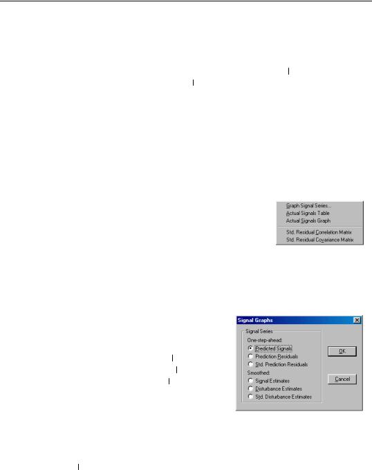
When you click on View/Signal Views, EViews displays a submenu containing additional view selections. Two of these selections are always available, even if the state space model has not yet been estimated:
•Actual Signal Table and Actual Signal Graph display the dependent signal variables in spreadsheet and graphical forms, respectively. If there are multiple signal equations, EViews will display a each series with its own axes.
The remaining views are only available following estimation.
•Graph Signal Series... opens a dialog with choices for the results to be displayed. The dialog allows you to choose between the onestep ahead predicted signals, yt t − 1 , the cor-
responding one-step residuals, t t − 1 , or standardized one-step residuals, et t − 1 , the
smoothed signals, ˆ t , smoothed signal distur- y
bances, ˆt , or the standardized smoothed sig-
nal disturbances, ˆ t . ± (root mean square) e 2
standard error bands are plotted where appropriate.
•Std. Residual Correlation Matrix and Std. Residual Covariance Matrix display the correlation and covariance matrix of the standardized one-step ahead signal residual, et t − 1 .
Working with the State Space—771
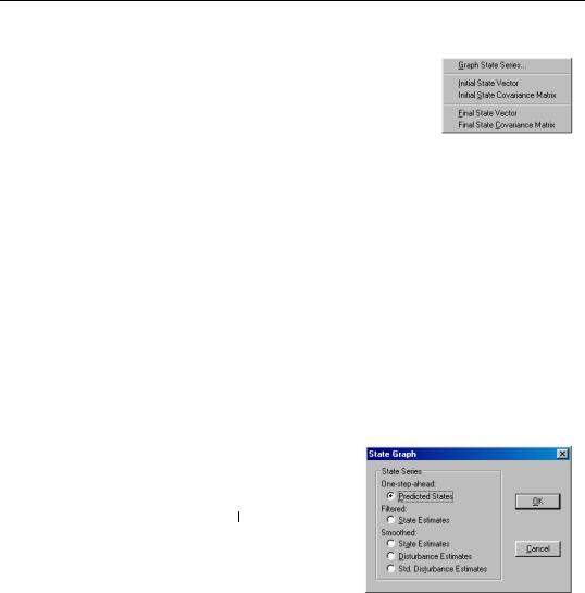
State Views
To examine the unobserved state components, click on View/ State Views to display the state submenu. EViews allows you to examine the initial or final values of the state components, or to graph the full time-path of various filtered or smoothed state data.
Two of the views are available either before or after estimation:
•Initial State Vector and Initial State Covariance Matrix display the values of the
initial state vector, α0 , and covariance matrix, P0 . If the unknown parameters have previously been estimated, EViews will evaluate the initial conditions using the esti-
mated values. If the sspace has not been estimated, the current coefficient values will be used in evaluating the initial conditions.
This information is especially relevant in models where EViews is using the current values of the system matrices to solve for the initial conditions. In cases where you are having difficulty starting your estimation, you may wish to examine the values of the initial conditions at the starting parameter values for any sign of problems.
The remainder of the views are only available following successful estimation:
•Final State Vector and Final State Covariance Matrix display the values of the final state vector, αT , and covariance matrix, PT , evaluated at the estimated parameters.
•Select Graph State Series... to display a dialog containing several choices for the state information. You can graph the one-step ahead predicted states, at t − 1 , the filtered
(contemporaneous) states, at , the smoothed
state estimates, ˆ t , smoothed state distur-
α
bance estimates, ˆ t , or the standardized v
smoothed state disturbances, ˆ t . In each
η
case, the data are displayed along with corresponding ±2 standard error bands.
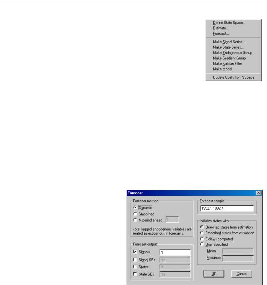
State Space Procedures
You can use the EViews procedures to create, estimate, forecast, and generate data from your state space specification. Select Proc in the sspace toolbar to display the available procedures:
772—Chapter 25. State Space Models and the Kalman Filter
•Define State Space... calls up the Auto-Specification dialog (see “Auto-Specification” on page 766). This feature provides a method of specifying a variety of common state space specifications using interactive menus.
•Select Estimate... to estimate the parameters of the specification (see “Estimating a State Space Model” on page 767).
These above items are available both before and after estimation. The automatic specification tool will replace the existing state space specification and will clear any results.
Once you have estimated your sspace, EViews provides additional tools for generating data:
•The Forecast... dialog allows you to generate forecasts of the states, signals, and the associated standard errors using alternative methods and initialization approaches.
First, select the forecast method. You can select between dynamic, smoothed, and n-period ahead forecasting, as described in “Forecasting” on page 756. Note that any lagged endogenous variables on the right-hand side of your signal equations will be treated as predetermined for purposes of forecasting.
EViews allows you to save various types of forecast output in series in your workfile. Simply check any of the output boxes, and specify the names for the series in the corresponding edit field.
You may specify the names either as a list or using a wildcard expression. If you choose to list the names, the number of identifiers must match the
number of signals in your specification. You should be aware that if an output series with a specified name already exists in the workfile, EViews will overwrite the entire contents of the series.
If you use a wildcard expression, EViews will substitute the name of each signal in the appropriate position in the wildcard expression. For example, if you have a model with signals Y1 and Y2, and elect to save the one-step predictions in “PRED*”, EViews will use the series PREDY1 and PREDY2 for output. There are two limitations to this feature: (1) you may not use the wildcard expression “*” to save

Working with the State Space—773
signal results since this will overwrite the original signal data, and (2) you may not use a wildcard when any signal dependent variables are specified by expression, or when there are multiple equations for a signal variable. In both cases, EViews will be unable to create the new series and will generate an error message.
Keep in mind that if your signal dependent variable is an expression, EViews will only provide forecasts of the expression. Thus, if your signal variable is LOG(Y), EViews will forecast the logarithm of Y.
Now enter a sample and specify the treatment of the initial states, and then click OK. EViews will compute the forecast and will place the results in the specified series. No output window will open.
There are several options available for setting the initial conditions. If you wish, you can instruct the sspace object to use the One-step ahead or Smoothed estimates of the state and state covariance as initial values for the forecast period. The two initialization methods differ in the amount of information used from the estimation sample; one-step ahead uses information up to the beginning of the forecast period, while smoothed uses the entire estimation period.
Alternatively, you may use EViews computed initial conditions. As in estimation, if possible, EViews will solve the Algebraic Riccati equations to obtain values for the initial state and state covariance at the start of each forecast interval. If solution of these conditions is not possible, EViews will use diffuse priors for the initial values.
Lastly, you may choose to provide a vector and sym object which contain the values for the forecast initialization. Simply select User Specified and enter the name of valid EViews objects in the appropriate edit fields.
Note that when performing either dynamic or smoothed forecasting, EViews requires that one-step ahead and smoothed initial conditions be computed from the estimation sample. If you choose one of these two forecasting methods and your forecast period begins either before or after the estimation sample, EViews will issue an error and instruct you to select a different initialization method.
When computing n-step ahead forecasting, EViews will adjust the start of the forecast period so that it is possible to obtain initial conditions for each period using the specified method. For the one-step ahead and smoothed methods, this means that at the earliest, the forecast period will begin n − 1 observations into the estimation sample, with earlier forecasted values set to NA. For the other initialization methods, forecast sample endpoint adjustment is not required.
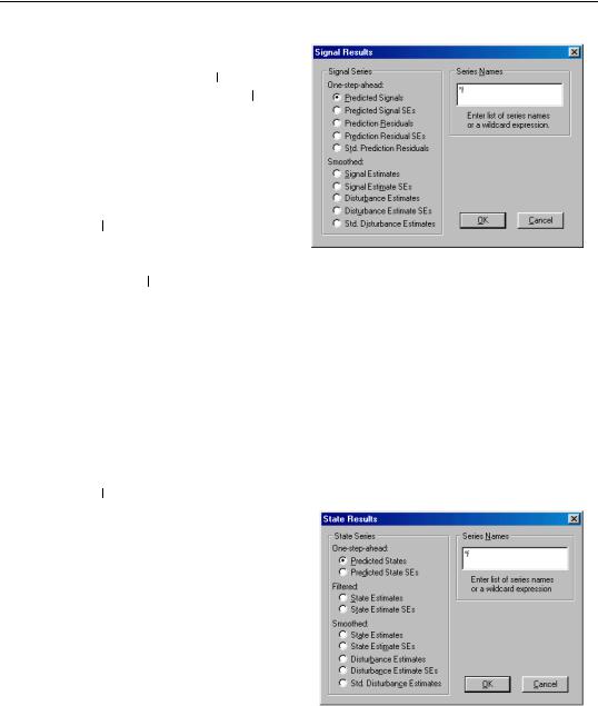
•Make Signal Series... allows you to create series containing various signal results computed over the estimation sample. Simply click on the menu entry to display the results dialog.
774—Chapter 25. State Space Models and the Kalman Filter
You may select the one-step ahead
predicted signals, ˜ t t − 1 , one- yy
step prediction residuals, t t − 1 ,
smoothed signal, ˆ t , or signal dis- y
turbance estimates, ˆt . EViews
also allows you to save the corresponding standard errors for each of these components (square roots of the diagonal elements of
ˆ
Ft t − 1 , St , and Ωt ), or the standardized values of the one-step residuals and smoothed disturbances, et t − 1
Next, specify the names of your series in the edit field using a list or wildcards as described above. Click OK to generate a group containing the desired signal series.
As above, if your signal dependent variable is an expression, EViews will only export results based upon the entire expression.
•Make State Series... opens a dialog allowing you to create series containing results for the state variables computed over the estimation sample. You can choose to save
either the one-step ahead state estimate, at |
|
t − 1 , the filtered state mean, at , the |
|
|
|
|
|||
ˆ |
ˆ |
|
ˆ |
, or |
smoothed states, αt , state disturbances, |
vt , standardized state disturbances, ηt |
|||
the corresponding standard error series (square roots of the diagonal elements of
ˆ
Pt t − 1 , Pt , Vt and Ωt ).
Simply select one of the output types, and enter the names of the output series in the edit field. The rules for specifying the output names are the same as for the Forecast...
procedure described above. Note that the wildcard expression “*” is permitted when saving state results. EViews will simply use the state names defined in your specification.
We again caution you that if an out-
put series exists in the workfile, EViews will overwrite the entire contents of the series.
•Click on Make Endogenous Group to create a group object containing the signal dependent variable series.