The @OBSNUM keyword allows you to number the observations in the workfile in sequential order from 1 to the total number of observations.
Working with Panel Data
For the most part, you will find working with data in a panel workfile to be identical to working with data in any other workfile. There are, however, some differences in behavior that require discussion. In addition, we describe useful approaches to working with panel data using standard, non panel-specific tools.
Lags and Leads
For the most part, expressions involving lags and leads should operate as expected (see “Lags, Leads, and Panel Structured Data” on page 212 for a full discussion). In particular note that lags and leads do not cross group boundaries so that they will never involve data from a different cross-section (i.e., lags of the first observation in a cross-section are always NAs, as are leads of the last observation in a cross-section).
Since EViews automatically sorts your data by cross-section and cell/date ID, observations in a panel dataset are always stacked by cross-section, with the cell IDs sorted within each cross-section. Accordingly, lags and leads within a cross-section are defined over the sorted values of the cell ID. Lags of an observation are always associated with lower value of the cell ID, and leads always involve a higher value (the first lag observation has the next lowest cell ID value and the first lead has the next highest value).
Lags and leads are specified in the usual fashion, using an offset in parentheses. To assign the sum of the first lag of Y and the second lead of X to the series Z, you may use the command:
series z = y(-1) + x(2)
Similarly, you may use lags to obtain the name of the previous child in household crosssections. The command:
alpha older = childname(-1)
assigns to the alpha series OLDER the name of the preceding observation. Note that since lags never cross over cross-section boundaries, the first value of OLDER in a household will be missing.
Panel Samples
The description of the current workfile sample in the workfile window provides an obvious indication that samples for dated and undated workfiles are specified in different ways.
882—Chapter 28. Working with Panel Data
Dated Panel Samples
For dated workfiles, you may specify panel samples using date pairs to define the earliest and latest dates to be included. For example, in our dated panel example from above, if we issue the sample statement:
smpl 1940 1954
EViews will exclude all observations that are dated from 1935 through 1939. We see that the new sample has eliminated observations for those dates from each cross-section.
As in non-panel workfiles, you may combine the date specification with additional “if” conditions to exclude additional observations. For example:
smpl 1940 1945 1950 1954 if i>50
uses any panel observations that are dated from 1940 to 1945 or 1950 to 1954 that have values of the series I that are greater than 50.
Additionally, you may use special keywords to refer to the first and last observations for cross-sections. For dated panels, the sample keywords @FIRST and @LAST refer to the set of first and last observations for each cross-section. For example, you may specify the sample:
smpl @first 2000
to use data from the first observation in each cross-section and observations up through the end of the year 2000. Likewise, the two sample statements:
smpl @first @first+5
smpl @last-5 @last
use (at most) the first five and the last five observations in each cross-section, respectively.
Note that the included observations for each cross-section may begin at a different date, and that:
smpl @all
smpl @first @last
are equivalent.
Working with Panel Data—883
The sample statement keywords @FIRSTMIN and @LASTMAX are used to refer to the earliest of the start and latest of the end dates observed over all cross-sections, so that the sample:
smpl @firstmin @firstmin+20
sets the start date to the earliest observed date, and includes the next 20 observations in each cross-section. The command:
smpl @lastmax-20 @lastmax
includes the last observed date, and the previous 20 observations in each cross-section.
Similarly, you may use the keywords @FIRSTMAX and @LASTMIN to refer to the latest of the cross-section start dates, and earliest of the end dates. For example, with regular annual data that begin and end at different dates, you may balance the starts and ends of your data using the statement:
smpl @firstmax @lastmin
which sets the sample to begin at the latest observed start date, and to end at the earliest observed end date.
The special keywords are perhaps most usefully combined with observation offsets. By adding plus and minus terms to the keywords, you may adjust the sample by dropping or adding observations within each cross-section. For example, to drop the first observation from each cross-section, you may use the sample statement:
smpl @first+1 @last
The following commands generate a series containing cumulative sums of the series X for each cross-section:
smpl @first @first
series xsum = x
smpl @first+1 @last
xsum = xsum(-1) + x
The first two commands initialize the cumulative sum for the first observation in each cross-section. The last two commands accumulate the sum of values of X over the remaining observations.
Similarly, if you wish to estimate your equation on a subsample of data and then perform cross-validation on the last 20 observations in each cross-section, you may use the sample defined by,
884—Chapter 28. Working with Panel Data
smpl @first @last-20
to perform your estimation, and the sample,
smpl @last-19 @last
to perform your forecast evaluation.
Note that the processing of sample offsets for each cross-section follows the same rules as for non-panel workfiles “Sample Offsets” on page 99.
Undated Panel Samples
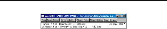
For undated workfiles, you must specify the sample range pairs using observation numbers defined over the entire workfile. For example, in our undated 506 observation panel example, you may issue the sample statement:
smpl 10 500
to drop the first 9 and the last 6 observations in the workfile from the current sample.
One consequence of the use of observation pairs in undated panels is that the keywords “@FIRST”, “@FIRSTMIN”, and “@FIRSTMAX” all refer to observation 1, and “@LAST”, “@LASTMIN”, and “@LASTMAX”, refer to the last observation in the workfile. Thus, in our example, the command:
smpl @first+9 @lastmax-6
will also drop the first 9 and the last 6 observations in the workfile from the current sample.
Undated panel sample restrictions of this form are not particularly interesting since they require detailed knowledge of the pattern of observation numbers across those cross-sec- tions. Accordingly, most sample statements in undated workfiles will employ “IF conditions” in place of range pairs.
For example, the sample statement,
smpl if townid<>10 and lstat >-.3
is equivalent to either of the commands,
smpl @all if townid<>10 and lstat >-.3 smpl 1 506 if townid<>10 and lstat >-.3
and selects all observations with TOWNID values not equal to 10, and LSTAT values greater than -0.3.
Working with Panel Data—885
You may combine the sample “IF conditions” with the special functions that return information about the observations in the panel. For example, we may use the “@OBSID” workfile function to identify each observation in a cross-section, so that:
smpl if @obsid>1
drops the first observation for each cross-section.
Alternately, to drop the last observation in each cross-section, you may use:
smpl if @obsid < @maxsby(townid, townid, "@all")
The @MAXSBY function returns the number of non-NA observations for each TOWNID value. Note that we employ the “@ALL” sample to ensure that we compute the @MAXSBY over the entire workfile sample.
Trends
EViews provides several functions that may be used to construct a time trend in your panel structured workfile. A trend in a panel workfile has the property that the values are initialized at the start of a cross-section, increase for successive observations in the specific cross-section, and are reset at the start of the next cross section.
You may use the following to construct your time trend:
•The @OBSID function may be used to return the simplest notion of a trend in which the values for each cross-section begin at one and increase by one for successive observations in the cross-section.
•The @TRENDC function computes trends in which values for observations with the earliest observed date are normalized to zero, and values for successive observations are incremented based on the calendar associated with the workfile frequency.
•The @CELLID and @TREND functions return time trends in which the values increase based on a calender defined by the observed dates in the workfile.
See also “Trend Functions” on page 592 and “Panel Trend Functions” on page 593 for discussion.
886—Chapter 28. Working with Panel Data
By-Group Statistics
The “by-group” statistical functions (“By-Group Statistics” on page 579) may be used to compute the value of a statistic for observations in a subgroup, and to assign the computed value to individual observations.
While not strictly panel functions, these tools deserve a place in the current discussion since they are well suited for working with panel data. To use the by-group statistical functions in a panel context, you need only specify the group ID series as the classifier series in the function.
Suppose, for example, that we have the undated panel structured workfile with the group ID series TOWNID, and that you wish to assign to each observation in the workfile the mean value of LSTAT in the corresponding town. You may perform the series assignment using the command,
series meanlstat = @meansby(lstat, townid, "@all")
or equivalently,
series meanlstat = @meansby(lstat, @crossid, "@all")
to assign the desired values. EViews will compute the mean value of LSTAT for observations with each TOWNID (or equivalently @CROSSID, since the workfile is structured using TOWNID) value, and will match merge these values to the corresponding observations.
Likewise, we may use the by-group statistics functions to compute the variance of LSTAT or the number of non-NA values for LSTAT for each subgroup using the assignment statements:
series varlstat = @varsby(lstat, townid, "@all")
series nalstat = @nasby(lstat, @crossid, "@all")
To compute the statistic over subsamples of the workfile data, simply include a sample string or object as an argument to the by-group statistic, or set the workfile sample prior to issuing the command,
smpl @all if zn=0
series meanlstat1 = @meansby(lstat, @cellid) is equivalent to,
smpl @all
series meanlstat2 = @meansby(lstat, @cellid, "@all if zn=0")
Working with Panel Data—887
In the former example, the by-group function uses the workfile sample to compute the statistic for each cell ID value, while in the latter, the optional argument explicitly overrides the workfile sample.
One important application of by-group statistics is to compute the “within” deviations for a series by subtracting off panel group means or medians. The following lines:
smpl @all
series withinlstat1 = lstat - @meansby(lstat, townid)
series withinlstat2 = lstat - @mediansby(lstat, townid)
compute deviations from the TOWNID specific means and medians. In this example, we omit the optional sample argument from the by-group statistics functions since the workfile sample is previously set to use all observations.
Combined with standard EViews tools, the by-group statistics allow you to perform quite complex calculations with little effort. For example, the panel “within” standard deviation for LSTAT may be computed from the single command:
The first line sets the sample to the first observation in each cross-section. The second line calculates the standard deviation of the group means using the single cross-sectional observations. Note that the group means are calculated over the entire sample. An alternative approach to performing this calculation is described in the next section.
Cross-section and Period Summaries
One of the most important tasks in working with panel data is to compute and save summary data, for example, computing means of a series by cross-section or period. In “ByGroup Statistics” on page 886, we outlined tools for computing by-group statistics using the cross-section ID and match merging them back into the original panel workfile page.
Additional tools are available for displaying tables summarizing the by-group statistics or for saving these statistics into new workfile pages.
888—Chapter 28. Working with Panel Data
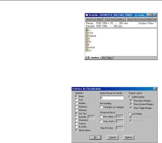
In illustrating these tools, we will work with the familiar Grunfeld data containing data on R&D expenditure and other economic measures for 10 firms for the years 1935 to 1954. These 200 observations form a balanced annual workfile that is structured using the firm number FN as the cross-section ID series, and the date series DATEID to identify the year.
Viewing Summaries
The easiest way to compute by-group statistics is to use the standard by-group statistics view of a series. Simply open the series window and select View/Descriptive Statistics/ Stats by Classification... to open the Statistics by Classification dialog.
First, you should enter the classifier series in the Series/Group to classify edit field. Here, we use FN, so that EViews will compute means, standard deviations, and number of observations for each cross-section in the panel workfile. Note that we have unchecked the Group into bins options so that EViews will not combine periods. The result of this computation for the series F is given by:
Working with Panel Data—889
Descriptive Statistics for F
Categorized by values of FN
Date: 02/04/04 Time: 15:26
Sample (adjusted): 1935 1954
Included observations: 200 after adjustments
FN
Mean
Std. Dev.
Obs.
1
4333.845
904.3048
20
2
1971.825
301.0879
20
3
1941.325
413.8433
20
4
693.2100
160.5993
20
5
231.4700
73.84083
20
6
419.8650
217.0098
20
7
149.7900
32.92756
20
8
670.9100
222.3919
20
9
333.6500
77.25478
20
10
70.92100
9.272833
20
All
1081.681
1314.470
200
Alternately, to compute statistics for each period in the panel, you should enter “DATEID” instead of “FN” as the classifier series.
Saving Summaries
Alternately, you may wish to compute the by-group panel statistics and save them in their own workfile page. The standard EViews tools for working with workfiles and creating series links make this task virtually effortless.
Creating Pages for Summaries
Since we will be computing both by-firm and by-period descriptive statistics, the first step is to create workfile pages to hold the results from our two sets of calculations. The firm page will contain observations corresponding to the unique values of the firm identifier found in the panel page; the annual page will contain observations corresponding to the observed years.
890—Chapter 28. Working with Panel Data
To create a page for the firm data, click on the New Page tab in the workfile window, and select Specify by Identifier series.... EViews opens the Workfile Page Create by ID dialog, with the identifiers prefilled with the series used in the panel workfile structure—the Date series field contains the name of the series used to identify dates in the panel, while the Cross-section ID series field contains the name of the series used to identify firms.
To create a new workfile using only the values in the FN series, you should delete the Date series
specification “DATEID” from the dialog. Next, provide a name for the new page by entering “firm” in the Page edit field. Now click on OK.
EViews will examine the FN series to find its unique values, and will create and structure a workfile page to hold those values.
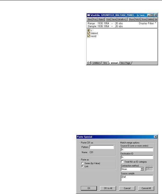
Here, we see the newly created FIRM page and newly created FN series containing the unique values from FN in the other page. Note that the new page is structured as an Undated with ID series page, using the new FN series.
Working with Panel Data—891
Repeating this process using the DATEID series will create an annual page. First click on the original panel page to make it active, then select New Page/Specify by Identifier series... to bring up the previous dialog. Delete the Cross-section ID series specification “FN” from the dialog, provide a name for the new page by entering “annual” in the Page edit field, and click on OK. EViews creates the third page, a regular frequency annual page dated 1935 to 1954.
Computing Summaries using Links
Once the firm and annual pages have been created, it is a simple task to create by-group summaries of the panel data using series links. While links are described elsewhere in greater depth (Chapter 8, “Series Links”, on page 177), we provide a brief description of their use in a panel data context.
To create links containing the desired summaries, first click on the original panel page tab to make it active, select one or more series of interest, then right mouse click and select Copy. Next, click on either the firm or the annual page, right mouse click, and select Paste Special.... EViews will open the Link Dialog, prompting you to specify a method for summarizing the data.
Suppose, for example, that you select and copy the C01, F, and I series from the panel page and then select Paste Special... in the firm page. EViews analyzes the two pages and prefills the Source ID and Destination ID series with two FN cross-section ID series.
You may provide a different pattern to be used in naming the link series, a contraction method, and a sample over which the contraction should be calculated. Here, we cre-
ate new series with the same names as the originals, computing means over the entire sample in the panel page. Click on OK to All to link all three series into the firm page, yielding:
892—Chapter 28. Working with Panel Data
You may compute other summary statistics by repeating the copy-and-paste-special procedure using alternate contraction methods. For example, selecting the Standard Deviation contraction computes the standard deviation for each cross-section and specified series and uses the linking to merge the results into the firm page. Saving them using the pattern “*SD” will create links named “C01SD”, “FSD”, and “ISD”.
Likewise, to compute summary statistics across cross-sections for each year, first create an annual page using New Page/Specify by Identifier series..., then paste-special the panel page series as links in the annual page.
Merging Data into the Panel
To merge data into the panel, simply create links from other pages into the panel page. Linking from the annual page into the panel page will repeat observations for each year across firms. Similarly, linking from the cross-section firm page to the panel page will repeat observations for each firm across all years.
In our example, we may link the FSD link from the firm page back into the panel page. Select FSD, switch to the panel page, and paste-special. Click OK to accept the defaults in the Paste Special dialog.
EViews match merges the data from the firm page to the panel page, matching FN values. Since the merge is from one-to-many, EViews simply repeats the values of FSD in the panel page.