Empirical research is usually an interactive process. The process begins with a specification of the relationship to be estimated. Selecting a specification usually involves several choices: the variables to be included, the functional form connecting these variables, and if the data are time series, the dynamic structure of the relationship between the variables.
Inevitably, there is uncertainty regarding the appropriateness of this initial specification. Once you estimate your equation, EViews provides tools for evaluating the quality of your specification along a number of dimensions. In turn, the results of these tests influence the chosen specification, and the process is repeated.
This chapter describes the extensive menu of specification test statistics that are available as views or procedures of an equation object. While we attempt to provide you with sufficient statistical background to conduct the tests, practical considerations ensure that many of the descriptions are incomplete. We refer you to standard statistical and econometric references for further details.
Background
Each test procedure described below involves the specification of a null hypothesis, which is the hypothesis under test. Output from a test command consists of the sample values of one or more test statistics and their associated probability numbers (p-values). The latter indicate the probability of obtaining a test statistic whose absolute value is greater than or equal to that of the sample statistic if the null hypothesis is true. Thus, low p-values lead to the rejection of the null hypothesis. For example, if a p-value lies between 0.05 and 0.01, the null hypothesis is rejected at the 5 percent but not at the 1 percent level.
Bear in mind that there are different assumptions and distributional results associated with each test. For example, some of the test statistics have exact, finite sample distributions (usually t or F-distributions). Others are large sample test statistics with asymptotic
χ2 distributions. Details vary from one test to another and are given below in the description of each test.
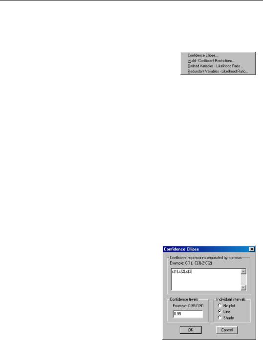
The View button on the equation toolbar gives you a choice among three categories of tests to check the specification of the equation.
Additional tests are discussed elsewhere in the User’s Guide. These tests include unit root tests (“Performing Unit Root Tests in EViews” on page 518), the Granger causality test (“Granger Causality” on
page 388), tests specific to binary, order, censored, and count models (Chapter 21, “Discrete and Limited Dependent Variable Models”, on page 621), and the Johansen test for cointegration (“How to Perform a Cointegration Test” on page 740).
570—Chapter 19. Specification and Diagnostic Tests
Coefficient Tests
These tests evaluate restrictions on the estimated coefficients, including the special case of tests for omitted and redundant variables.
Confidence Ellipses
The confidence ellipse view plots the joint confidence region of any two functions of estimated parameters from an EViews estimation object. Along with the ellipses, you can choose to display the individual confidence intervals.
We motivate our discussion of this view by pointing out that the Wald test view (View/ Coefficient Tests/Wald - Coefficient Restrictions...) allows you to test restrictions on the estimated coefficients from an estimation object. When you perform a Wald test, EViews provides a table of output showing the numeric values associated with the test.
An alternative approach to displaying the results of a Wald test is to display a confidence interval. For a given test size, say 5%, we may display the one-dimensional interval within which the test statistic must lie for us not to reject the null hypothesis. Comparing the realization of the test statistic to the interval corresponds to performing the Wald test.
The one-dimensional confidence interval may be generalized to the case involving two restrictions, where we form a joint confidence region, or confidence ellipse. The confidence ellipse may be interpreted as the region in which the realization of two test statistics must lie for us not to reject the null.
To display confidence ellipses in EViews, simply select View/Coefficient Tests/Confidence Ellipse... from the estimation object toolbar. EViews will display a dialog prompting you to specify the coefficient restrictions and test size, and to select display options.
The first part of the dialog is identical to that found in the Wald test view—here, you will enter your coefficient restrictions into the edit box, with multiple restrictions separated by commas. The computation of the confidence ellipse requires a minimum of two restrictions. If you provide more than two restrictions, EViews will display all unique pairs of confidence ellipses.
In this simple example depicted here, we provide a (comma separated) list of coefficients from the estimated equation. This description of the restrictions takes advantage of the fact that EViews interprets
any expression without an explicit equal sign as being equal to zero (so that “C(1)” and
.75
.70
.65
Coefficient Tests—571
“C(1)=0” are equivalent). You may, of course, enter an explicit restriction involving an equal sign (for example, “C(1)+C(2) = C(3)/2”).
Next, select a size or sizes for the confidence ellipses. Here, we instruct EViews to construct a 95% confidence ellipse. Under the null hypothesis, the test statistic values will fall outside of the corresponding confidence ellipse 5% of the time.
Lastly, we choose a display option for the individual confidence intervals. If you select Line or Shade, EViews will mark the confidence interval for each restriction, allowing you to see, at a glance, the individual results. Line will display the individual confidence intervals as dotted lines; Shade will display the confidence intervals as a shaded region. If you select None, EViews will not display the individual intervals.
The output depicts three confidence ellipses that result from pairwise tests implied by the three restrictions (“C(1)=0”, “C(2)=0”, and “C(3)=0”).
Notice first the presence of the dotted lines showing the corresponding confidence intervals for the individual coefficients.
The next thing that jumps out from this example is that the coefficient estimates are highly correlated—if the estimates were independent, the ellipses would be exact circles.
C(1)=0 (since it falls below the end of the univariate confidence interval). If C(3)=.8, we cannot reject the joint null that C(1)=0, and C(3)=0 (since C(1)=-.65, C(3)=.8 falls within the confidence ellipse).
EViews allows you to display more than one size for your confidence ellipses. This feature allows you to draw confidence contours so that you may see how the rejection region changes at different probability values. To do so, simply enter a space delimited list of confidence levels. Note that while the coefficient restriction expressions must be separated by commas, the contour levels must be separated by spaces.
572—Chapter 19. Specification and Diagnostic Tests
.85
.80
.75
C(3)
.70
.65
.60
.55
.50
-.022
-.020
-.018 -.016 -.014 -.012 -.010
C(2)
Here, the individual confidence intervals are depicted with shading. The individual intervals are based on the largest size confidence level (which has the widest interval), in this case, 0.9.
Computational Details
Consider two functions of the parameters f1( β) and f2( β) , and define the bivariate function f( β) = ( f1( β), f2( β) ) .
The size α joint confidence ellipse is defined as the set of points b such that:
ˆ
ˆ
−1
ˆ
(19.1)
( b − f( β) ) ′( V( β)
) ( b − f( β) ) = cα
ˆ
ˆ
ˆ
is the
where β
are the parameter estimates, V( β) is the covariance matrix of β , and cα
size α critical value for the related distribution. If the parameter estimates are leastsquares based, the F( 2, n − 2 ) distribution is used; if the parameter estimates are likelihood based, the χ2( 2 ) distribution will be employed.
The individual intervals are two-sided intervals based on either the t-distribution (in the cases where cα is computed using the F-distribution), or the normal distribution (where cα is taken from the χ2 distribution).
Wald Test (Coefficient Restrictions)
The Wald test computes a test statistic based on the unrestricted regression. The Wald statistic measures how close the unrestricted estimates come to satisfying the restrictions under the null hypothesis. If the restrictions are in fact true, then the unrestricted estimates should come close to satisfying the restrictions.
Coefficient Tests—573
How to Perform Wald Coefficient Tests
To demonstrate the calculation of Wald tests in EViews, we consider simple examples. Suppose a Cobb-Douglas production function has been estimated in the form:
log Q = A + αlog L + βlog K + ,
(19.2)
where Q , K and L denote value-added output and the inputs of capital and labor respectively. The hypothesis of constant returns to scale is then tested by the restriction:
α + β = 1 .
Estimation of the Cobb-Douglas production function using annual data from 1947 to 1971 provided the following result:
Dependent Variable: LOG(Q)
Method: Least Squares
Date: 08/11/97 Time: 16:56
Sample: 1947 1971
Included observations: 25
Variable
Coefficient
Std. Error
t-Statistic
Prob.
C
-2.327939
0.410601
-5.669595
0.0000
LOG(L)
1.591175
0.167740
9.485970
0.0000
LOG(K)
0.239604
0.105390
2.273498
0.0331
R-squared
0.983672
Mean dependent var
4.767586
Adjusted R-squared
0.982187
S.D. dependent var
0.326086
S.E. of regression
0.043521
Akaike info criterion
-3.318997
Sum squared resid
0.041669
Schwarz criterion
-3.172732
Log likelihood
44.48746
F-statistic
662.6819
Durbin-Watson stat
0.637300
Prob(F-statistic)
0.000000
The sum of the coefficients on LOG(L) and LOG(K) appears to be in excess of one, but to determine whether the difference is statistically relevant, we will conduct the hypothesis test of constant returns.
To carry out a Wald test, choose View/Coefficient Tests/Wald-Coefficient Restrictions… from the equation toolbar. Enter the restrictions into the edit box, with multiple coefficient restrictions separated by commas. The restrictions should be expressed as equations involving the estimated coefficients and constants. The coefficients should be referred to as C(1), C(2), and so on, unless you have used a different coefficient vector in estimation.
If you enter a restriction that involves a series name, EViews will prompt you to enter an observation at which the test statistic will be evaluated. The value of the series will at that period will be treated as a constant for purposes of constructing the test statistic.
To test the hypothesis of constant returns to scale, type the following restriction in the dialog box:
574—Chapter 19. Specification and Diagnostic Tests
c(2) + c(3) = 1
and click OK. EViews reports the following result of the Wald test:
Wald Test:
Equation: EQ1
Test Statistic
Value
df
Probability
Chi-square
120.0177
1
0.0000
F-statistic
120.0177
(1, 22)
0.0000
Null Hypothesis Summary:
Normalized Restriction (= 0)
Value
Std. Err.
-1 + C(2) + C(3)
0.830779
0.075834
Restrictions are linear in coefficients.
EViews reports an F-statistic and a Chi-square statistic with associated p-values. See “Wald Test Details” on page 576 for a discussion of these statistics. In addition, EViews reports the value of the normalized (homogeneous) restriction and an associated standard error. In this example, we have a single linear restriction so the two test statistics are identical, with the p-value indicating that we can decisively reject the null hypothesis of constant returns to scale.
To test more than one restriction, separate the restrictions by commas. For example, to test the hypothesis that the elasticity of output with respect to labor is 2/3 and the elasticity with respect to capital is 1/3, enter the restrictions as,
c(2)=2/3,
c(3)=1/3
and EViews reports:
Wald Test:
Equation: EQ1
Test Statistic
Value
df
Probability
Chi-square
53.99105
2
0.0000
F-statistic
26.99553
(2, 22)
0.0000
Null Hypothesis Summary:
Normalized Restriction (= 0)
Value
Std. Err.
-2/3 + C(2)
0.924508
0.167740
-1/3 + C(1)
-2.661272
0.410601
Restrictions are linear in coefficients.
Note that in addition to the test statistic summary, we report the values of both of the normalized restrictions, along with their standard errors (the square roots of the diagonal elements of the restriction covariance matrix).
Coefficient Tests—575
As an example of a nonlinear model with a nonlinear restriction, we estimate a production function of the form:
log Q = β1 + β2log ( β3Kβ4 + ( 1 − β3) Lβ4 ) +
(19.3)
and test the constant elasticity of substitution (CES) production function restriction
β2 = 1 ⁄ β4 . This is an example of a nonlinear restriction. To estimate the (unrestricted) nonlinear model, you should select Quick/Estimate Equation… and then enter the following specification:
To test the nonlinear restriction, choose View/Coefficient Tests/Wald-Coefficient Restrictions… from the equation toolbar and type the following restriction in the Wald Test dialog box:
c(2)=1/c(4)
The results are presented below:
Wald Test:
Equation: EQ2
Test Statistic
Value
df
Probability
Wald
Test:
0.028508
1
0.8659
Chi-square
Equation: EQ2
0.028508
(1, 21)
0.8675
F-statistic
Null
Hypothesis:
C(2)=1/C(4)
F-statisticNull Hypothesis Summary:0.028507
Probability
0.867539
Chi-square
0.028507
Probability
0.865923
Normalized Restriction (= 0)
Value
Std. Err.
C(2) - 1/C(4)
1.292163
7.653088
Delta method computed using analytic derivatives.
Since this is a nonlinear equation, we focus on the Chi-square statistic which fails to reject the null hypothesis. Note that EViews reports that it used the delta method (with analytic derivatives) to compute the Wald restriction variance for the nonlinear restriction.
It is well-known that nonlinear Wald tests are not invariant to the way that you specify the nonlinear restrictions. In this example, the nonlinear restriction β2 = 1 ⁄ β4 may equivalently be written as β2β4 = 1 or β4 = 1 ⁄ β2 (for nonzero β2 and β4 ). For example, entering the restriction as,
c(2)*c(4)=1
yields:
576—Chapter 19. Specification and Diagnostic Tests
Wald Test:
Equation: EQ2
Test Statistic
Value
df
Probability
Wald
Test:
104.5599
1
0.0000
Chi-square
Equation: EQ2
104.5599
(1, 21)
0.0000
F-statistic
Null
Hypothesis:
C(2)*C(4)=1
F-statisticNullHypothesis Summary:104.5599
Probability
0.000000
Chi-
square
104.5599
Probability
0.000000
Normalized Restriction (= 0)
Value
Std. Err.
-1 + C(2)*C(4)
0.835330
0.081691
Delta method computed using analytic derivatives.
so that the test now decisively rejects the null hypothesis. We hasten to add that type of inconsistency is not unique to EViews, but is a more general property of the Wald test. Unfortunately, there does not seem to be a general solution to this problem (see Davidson and MacKinnon, 1993, Chapter 13).
Wald Test Details
Consider a general nonlinear regression model:
y = f( β) +
(19.4)
where y and are T -vectors and β is a k -vector of parameters to be estimated. Any restrictions on the parameters can be written as:
H0: g( β) = 0 ,
(19.5)
where g is a smooth function, g: Rk → Rq , imposing q restrictions on β . The Wald statistic is then computed as:
W
= g( β) ′
∂g( β) ˆ
∂g( β)
g( β)
β = b
(19.6)
--------------V( b) --------------
∂β
∂β′
where T is the number of observations and b is the vector of unrestricted parameter esti-
ˆ
ˆ
mates, and where V is an estimate of the b covariance. In the standard regression case, V
is given by:
ˆ
= s
2
∂f( β) ∂f( β)
−1
(19.7)
V( b)
-------------- --------------
∂β ∂β′
β = b
where u is the vector of unrestricted residuals, and s2
is the usual estimator of the unre-
stricted residual variance, s2 = ( u′u) ⁄ ( N − k) , but the estimator of V may differ. For
ˆ
example, V may be a robust variance matrix estimator computing using White or NeweyWest techniques.
More formally, under the null hypothesis H0 , the Wald statistic has an asymptotic χ2( q) distribution, where q is the number of restrictions under H0 .
Coefficient Tests—577
For the textbook case of a linear regression model,
y = Xβ +
(19.8)
and linear restrictions:
H0: Rβ − r = 0 ,
(19.9)
where R is a known q × k matrix, and r is a q -vector, respectively. The Wald statistic in Equation (19.6) reduces to:
W = ( Rb − r) ′ ( Rs2( X′X) −1R′ )−1( Rb − r) ,
(19.10)
which is asymptotically distributed as χ2( q) under H0 .
If we further assume that the errors are independent and identically normally distrib-
uted, we have an exact, finite sample F-statistic:
W
( u′ u − u′u) ⁄ q
F = -----
=
˜ ˜
(19.11)
----------------------------------- ,
q
( u′u) ⁄ ( T − k)
where ˜ is the vector of residuals from the restricted regression. In this case, the -statis- u F
tic compares the residual sum of squares computed with and without the restrictions imposed.
We remind you that the expression for the finite sample F-statistic in (19.11) is for standard linear regression, and is not valid for more general cases (nonlinear models, ARMA specifications, or equations where the variances are estimated using other methods such as Newey-West or White). In non-standard settings, the reported F-statistic (which EViews always computes as W ⁄ q ), does not possess the desired finite-sample properties. In these cases, while asymptotically valid, the F-statistic results should be viewed as illustrative and for comparison purposes only.
Omitted Variables
This test enables you to add a set of variables to an existing equation and to ask whether the set makes a significant contribution to explaining the variation in the dependent variable. The null hypothesis H0 is that the additional set of regressors are not jointly significant.
The output from the test is an F-statistic and a likelihood ratio (LR) statistic with associated p-values, together with the estimation results of the unrestricted model under the alternative. The F-statistic is based on the difference between the residual sums of squares of the restricted and unrestricted regressions and is only valid in linear regression based settings. The LR statistic is computed as:
LR = −2( lr − lu)
(19.12)
578—Chapter 19. Specification and Diagnostic Tests
where lr and lu are the maximized values of the (Gaussian) log likelihood function of the unrestricted and restricted regressions, respectively. Under H0 , the LR statistic has an asymptotic χ2 distribution with degrees of freedom equal to the number of restrictions (the number of added variables).
Bear in mind that:
•The omitted variables test requires that the same number of observations exist in the original and test equations. If any of the series to be added contain missing observations over the sample of the original equation (which will often be the case when you add lagged variables), the test statistics cannot be constructed.
•The omitted variables test can be applied to equations estimated with linear LS, TSLS, ARCH (mean equation only), binary, ordered, censored, truncated, and count models. The test is available only if you specify the equation by listing the regressors, not by a formula.
To perform an LR test in these settings, you can estimate a separate equation for the unrestricted and restricted models over a common sample, and evaluate the LR statistic and p- value using scalars and the @cchisq function, as described above.
How to Perform an Omitted Variables Test
To test for omitted variables, select View/Coefficient Tests/Omitted Variables-Likelihood Ratio… In the dialog that opens, list the names of the test variables, each separated by at least one space. Suppose, for example, that the initial regression is:
ls log(q) c log(l) log(k)
If you enter the list:
log(m) log(e)
in the dialog, then EViews reports the results of the unrestricted regression containing the two additional explanatory variables, and displays statistics testing the hypothesis that the coefficients on the new variables are jointly zero. The top part of the output depicts the test results:
Omitted Variables: LOG(M) LOG(E)
F-statistic
4.267478
Probability
0.028611
Log likelihood ratio
8.884940
Probability
0.011767
The F-statistic has an exact finite sample F-distribution under H0 for linear models if the errors are independent and identically distributed normal random variables. The numerator degrees of freedom is the number of additional regressors and the denominator degrees of freedom is the number of observations less the total number of regressors. The log like-