Chapter 26. Models

A model in EViews is a set of one or more equations that jointly describe the relationship between a set of variables. The model equations can come from many sources: they can be simple identities, they can be the result of estimation of single equations, or they can be the result of estimation using any one of EViews’ multiple equation estimators.

EViews models allow you to combine equations from all these sources inside a single object, which may be used to create a deterministic or stochastic joint forecast or simulation for all of the variables in the model. In a deterministic setting, the inputs to the model are fixed at known values, and a single path is calculated for the output variables. In a stochastic environment, uncertainty is incorporated into the model by adding a random element to the coefficients, the equation residuals or the exogenous variables.

Models also allow you to examine simulation results under different assumptions concerning the variables that are determined outside the model. In EViews, we refer to these sets of assumptions as scenarios, and provide a variety of tools for working with multiple model scenarios.

Even if you are working with only a single equation, you may find that it is worth creating a model from that equation so that you may use the features provided by the EViews Model object.

Overview

The following section provides a brief introduction to the purpose and structure of the EViews model object, and introduces terminology that will be used throughout the rest of the chapter.

A model consists of a set of equations that describe the relationships between a set of variables.

The variables in a model can be divided into two categories: those determined inside the model, which we refer to as the endogenous variables, and those determined outside the model, which we refer to as the exogenous variables. A third category of variables, the add factors, are a special case of exogenous variables.

In its most general form, a model can be written in mathematical notation as:

Overview—779

variables, we may require a more complicated procedure to solve for the entire set of periods simultaneously.

In EViews, when solving a model, we must first associate data with each variable in the model by binding each of the model variables to a series in the workfile. We then solve the model for each observation in the selected sample and place the results in the corresponding series.

When binding the variables of the model to specific series in the workfile, EViews will often modify the name of the variable to generate the name of the series. Typically, this will involve adding an extension of a few characters to the end of the name. For example, an endogenous variable in the model may be called “Y”, but when EViews solves the model, it may assign the result into an observation of a series in the workfile called “Y_0”. We refer to this mapping of names as aliasing. Aliasing is an important feature of an EViews model, as it allows the variables in the model to be mapped into different sets of workfile series, without having to alter the equations of the model.

When a model is solved, aliasing is typically applied to the endogenous variables so that historical data is not overwritten. Furthermore, for models which contain lagged endogenous variables, aliasing allows us to bind the lagged variables to either the actual historical data, which we refer to as a static forecast, or to the values solved for in previous periods, which we refer to as a dynamic forecast. In both cases, the lagged endogenous variables are effectively treated as exogenous variables in the model when solving the model for a single period.

Aliasing is also frequently applied to exogenous variables when using model scenarios. Model scenarios allow you to investigate how the predictions of your model vary under different assumptions concerning the path of exogenous variables or add factors. In a scenario, you can change the path of an exogenous variable by overriding the variable. When a variable is overridden, the values for that variable will be fetched from a workfile series specific to that scenario. The name of the series is formed by adding a suffix associated with the scenario to the variable name. This same suffix is also used when storing the solutions of the model for the scenario. By using scenarios it is easy to compare the outcomes predicted by your model under a variety of different assumptions without having to edit the structure of your model.

The following table gives a typical example of how model aliasing might map variable names in a model into series names in the workfile:

An Example Model—781

•R is the interest rate on three-month treasury bills

•M is the real money supply, narrowly defined (M1)

and the C(i) are the unknown coefficients.

The model follows the structure of a simple textbook ISLM macroeconomic model, with expenditure equations relating consumption and investment to GDP and interest rates, and a money market equation relating interest rates to GDP and the money supply. The fourth equation is the national accounts expenditure identity which ensures that the components of GDP add to total GDP. The model differs from a typical textbook model in its more dynamic structure, with many of the variables appearing in lagged or differenced form.

To begin, we must first estimate the unknown coefficients in the stochastic equations. For simplicity, we estimate the coefficients by simple single equation OLS. Note that this approach is not strictly valid, since Y appears on the right-hand side of several of the equations as an independent variable but is endogenous to the system as a whole. Because of this, we would expect Y to be correlated with the residuals of the equations, which violates the assumptions of OLS estimation. To adjust for this, we would need to use some form of instrumental variables or system estimation (for details, see the discussion of single equation “Two-stage Least Squares” beginning on page 473 and system “Two-Stage Least Squares” and related sections beginning on page 697).

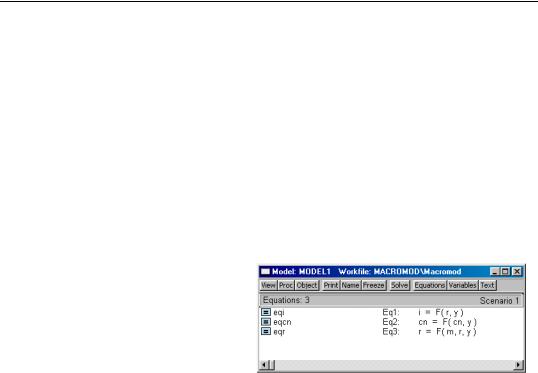
To estimate the equations in EViews, we create three new equation objects in the workfile (using Object/New Object.../Equation), and then enter the appropriate specifications. Since all three equations are linear, we can specify them using list form. To minimize confusion, we will name the three equations according to their endogenous variables. The resulting names and specifications are:

The three equations estimate satisfactorily and provide a reasonably close fit to the data, although much of the fit probably comes from the lagged endogenous variables. The consumption and investment equations show signs of heteroskedasticity, possibly indicating that we should be modeling the relationships in log form. All three equations show signs of serial correlation. We will ignore these problems for the purpose of this example, although you may like to experiment with alternative specifications and compare their performance.

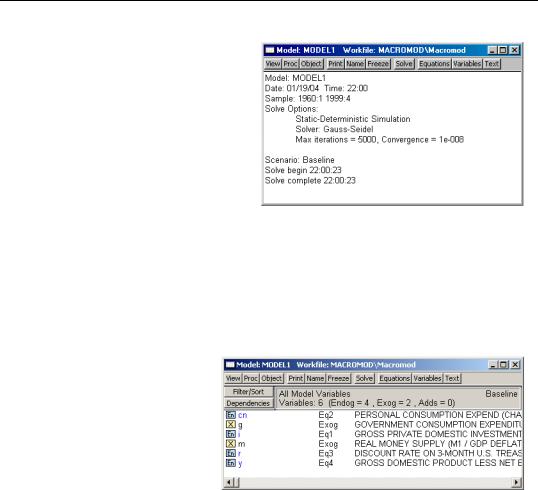
Now that we have estimated the three equations, we can proceed to the model itself. To create the model, we simply select Object/New Object.../Model from the menus. To keep the model permanently in the workfile, we name the model by clicking on the Name button, enter the name MODEL1, and click on OK.

An Example Model—783

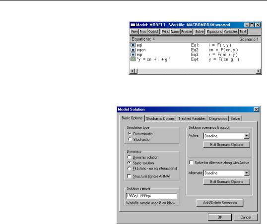
The equation should now appear in the model window. The appearance differs slightly from the other equations, which is an indicator that the new equation is an inline text equation rather than a link.

Our model specification is now com-

plete. At this point, we can proceed straight to solving the model. To solve the model, simply click on the Solve button in the model window button bar.

There are many options available from the dialog, but for the moment we will consider only the basic settings. As our first exercise in assessing our model, we would like to examine the ability of our model to provide one-period ahead forecasts of our endogenous variables. To do this, we can look at the predictions of our model against our historical data, using actual values for both the exogenous and the lagged endogenous variables of the model. In EViews, we refer to this as a static simula-

tion. We may easily perform this type of simulation by choosing Static solution in the Dynamics box of the dialog.

We must also adjust the sample over which to solve the model, so as to avoid initializing our solution with missing values from our data. Most of our series are defined over the range of 1947Q1 to 1999Q4, but our money supply series is available only from 1959Q1. Because of this, we set the sample to 1960Q1 to 1999Q4, allowing a few extra periods prior to the sample for any lagged variables.

We are now ready to solve the model. Simply click on OK to start the calculations. The model window will switch to the Solution Messages view.

An Example Model—785

and its associated procedures help you move between these different sets of series without having to worry about the many different names involved.

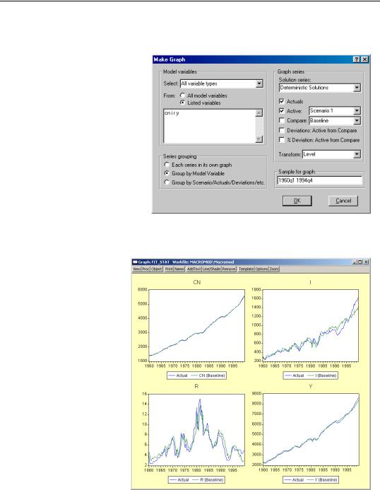
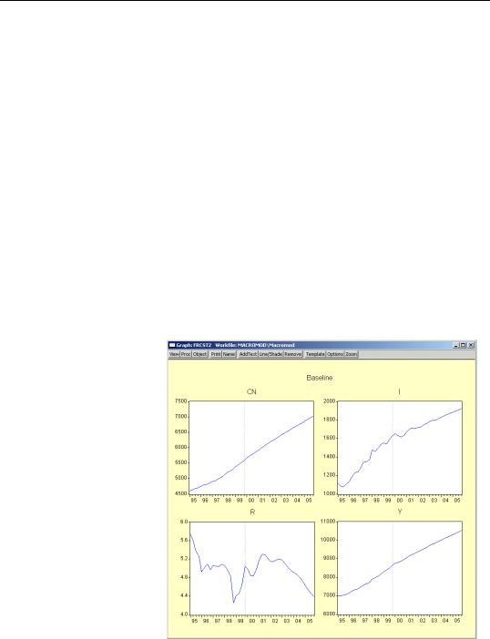
For example, to look at graphs containing the actual and fitted values for the endogenous variables in our model, we simply select the four variables (by holding down the control key and clicking on the variable names), then use Proc/ Make Graph… to enter the dialog.

Again, the dialog has many options, but for our current purposes, we can leave most

settings at their default values. Simply make sure that the Actuals and Active checkboxes are checked, set the sample for the graph to 1960Q1 to 1999Q4, then click on OK.

The graphs show that as a one-step ahead predictor, the model performs quite well, although the ability of the model to predict investment deteriorates during the second half of the sample.

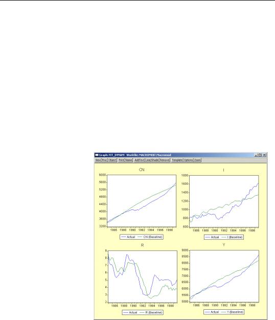
An alternative way of evaluating the model is to examine how the model performs when used to forecast many periods into the future. To do this, we must use our forecasts from previous periods, not actual historical data, when assigning values

An Example Model—787

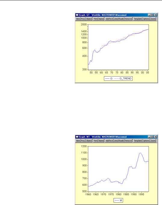
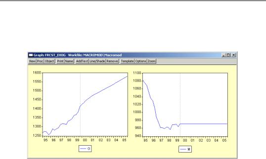
A quick look at our historical series for G suggests that the growth rate of G has been fairly constant since 1960, so that the log of G roughly follows a linear trend. Where G deviates from the trend, the deviations seem to follow a cyclical pattern.

As a simple model of this behavior, we can regress the log of G against a constant and a time trend, using an AR(4) error structure to model the cyclical deviations. This gives the following equation, which we save in the workfile as EQG:

log(g) = 6.252335363 + 0.004716422189*@trend + [ar(1)=1.169491542,ar(2)=0.1986105964,ar(3)=0.239913126,ar( 4)=-0.2453607091]

To produce a set of future values for G, we can use this equation to perform a dynamic forecast from 2000Q1 to 2005Q4, saving the results back into G itself (see page 797 for details).

The historical path of the real M1 money supply, M, is quite different from G, showing spurts of growth followed by periods of stability.

For now, we will assume that the real money supply simply remains at its last observed historical value over the entire forecast period.

We can use an EViews series statement to fill in this path. The following lines will fill the series M from 2000Q1 to the last observation in the sample with the last observed historical value for M:

smpl 2000q1 @last

series m = m(-1)

An Example Model—789

We observe strange behavior in the results. At the beginning of the forecast period, we see a heavy dip in investment, GDP, and interest rates. This is followed by a series of oscillations in these series with a period of about a year, which die out slowly during the forecast period. This is not a particularly convincing forecast.

There is little in the paths of our exogenous variables or the history of our endogenous variables that would lead to

this sharp dip, suggesting that the problem may lie with the residuals of our equations. Our investment equation is the most likely candidate, as it has a large, persistent positive residual near the end of the historical data (see figure below). This residual will be set to zero over the forecast period when solving the model, which might be the cause of the sudden drop in investment at the beginning of the forecast.

One way of dealing with this problem would be to change the specification of the investment equation. The simplest modification would be to add an autoregressive component to the equation, which would help reduce the persistence of the error. A better alternative would be to try to modify the variables in the equation so that the equation can provide some explanation for the sharp rise in investment during the 1990s.

An Example Model—791

sort of errors occurring in the future as we have seen in history. We have also been ignoring the fact that some of the coefficients in our equations are estimated, rather than fixed at known values. We may like to reflect this uncertainty about our coefficients in some way in the results from our model.

We can incorporate these features into our EViews model using stochastic simulation.

Up until now, we have thought of our model as forecasting a single point for each of our endogenous variables at each observation. As soon as we add uncertainty to the model, we should think instead of our model as predicting a whole distribution of outcomes for each variable at each observation. Our goal is to summarize these distributions using appropriate statistics.

If the model is linear (as in our example) and the errors are normal, then the endogenous variables will follow a normal distribution, and the mean and standard deviation of each distribution should be sufficient to describe the distribution completely. In this case, the mean will actually be equal to the deterministic solution to the model. If the model is not linear, then the distributions of the endogenous variables need not be normal. In this case, the quantiles of the distribution may be more informative than the first two moments, since the distributions may have tails which are very different from the normal case. In a non-linear model, the mean of the distribution need not match up to the deterministic solution of the model.

EViews makes it easy to calculate statistics to describe the distributions of your endogenous variables in an uncertain environment. To simulate the distributions, the model object uses a Monte Carlo approach, where the model is solved many times with pseudorandom numbers substituted for the unknown errors at each repetition. This method provides only approximate results. However, as the number of repetitions is increased, we would expect the results to approach their true values.

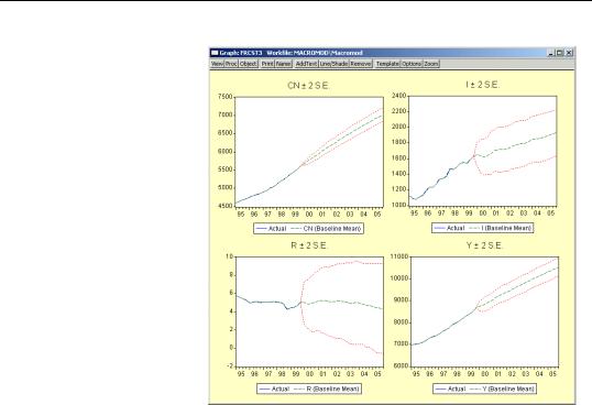
To return to our simple macroeconomic model, we can use a stochastic simulation to provide some measure of the uncertainty in our results by adding error bounds to our predictions. From the model window, click on the Solve button. When the model solution dialog appears, choose Stochastic for the simulation type. In the Solution scenarios & output box, make sure that the Std. Dev. checkbox in the Active section is checked. Click on OK to begin the simulation.

The simulation should take about half a minute. Status messages will appear to indicate progress through the repetitions. When the simulation is complete, you may return to the variable view, use the mouse to select the variables as discussed above, and then select Proc/Make Graph…. When the Make Graph dialog appears, select the option Mean +- 2 standard deviations in the Solution Series list box in the Graph Series area on the right of the dialog. Set the sample to 1995Q1 to 2005Q4 and click on OK.

An Example Model—793

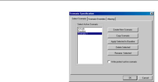
They differ in that the actuals scenario writes its solution values directly into the workfile series with the same names as the endogenous variables, while the baseline scenario writes its solution values back into workfile series with the extension “_0”.

To add a new scenario to the model, simply click on the button labeled Create new scenario. A new scenario will be created immediately. You can use this dialog to select which

scenario is currently active, or to rename and delete scenarios.

Once we have created the scenario, we can modify the scenario from the baseline case by overriding one of our exogenous variables. To do this, return to the variable window of the model, click on the variable M, use the right mouse button to call up the Properties dialog for the variable, and then in the Scenario box, click on the checkbox for Use override series in scenario. A message will appear asking if you would like to create the new series. Click on Yes to create the series, then OK to return to the variable window.

In the variable window, the variable name “M” should now appear in red, indicating that it has been overridden in the active scenario. This means that the variable M will now be bound to the series M_1 instead of the series M when solving the model. In our previous forecast for M, we assumed that the real money supply would be kept at a constant level during the forecast period. For our alternative scenario, we are going to assume that the real money supply is contracted sharply at the beginning of the forecast period, and held at this lower value throughout the forecast. We can set the new values using a few simple commands:

smpl 2000q1 2005q4

series m_1 = 900

smpl @all

As before, we can solve the model by clicking on the Solve button. Restore the Simulation type to deterministic, make sure that Scenario 1 is the active scenario, then click on OK. Once the solution is complete, we can use Proc/Make Graph… to display the results following the same procedure as above. Restore the Solution series list box to the setting Deterministic solutions, then check both the Active and Compare solution checkboxes