Добавил:
Upload Опубликованный материал нарушает ваши авторские права? Сообщите нам.
Вуз: Предмет: Файл:
Eviews5 / EViews5 / Docs / EViews 5 Users Guide.pdf
Скачиваний:
152
Добавлен:
23.03.2015
Размер:
11.51 Mб
Скачать

794—Chapter 26. Models

below, making sure that the active scenario is set to Scenario 1, and the comparison scenario is set to Baseline. Again set the sample to 1995Q1 to 2005Q4. The following graph should be displayed:

The simulation results suggest that the cut in the money supply causes a substantial increase in interest rates, which creates a small reduction in investment and a relatively minor drop in income and consumption. Overall, the predicted effects of changes in the money supply on the real economy are relatively minor in this model.

This concludes the discussion of our example model. The

remainder of this chapter provides detailed information about working with particular features of the EViews model object.

Building a Model

Creating a Model

The first step in working with a model is to create the model object itself. There are several different ways of creating a model:

You can create an empty model by using Object/New Object… and then choosing Model, or by performing the same operation using the right mouse button menu from inside the workfile window.

You can select a list of estimation objects in the workfile window (equations, VARs, systems), and then select Open as Model from the right mouse button menu. This item will create a model which contains the equations from the selected objects as links.

Building a Model—795

You can use the Make model procedure from an estimation object to create a model containing the equation or equations in that object.

Adding Equations to the Model

The equations in a model can be classified into two types: linked equations and inline equations. Linked equations are equations that import their specification from other objects in the workfile. Inline equations are contained inside the model as text.

There are a number of ways to add equations to your model:

To add a linked equation: from the workfile window, select the object which contains the equation or equations you would like to add to the model, then copy-and- paste the object into the model equation view window.

To add an equation using text: select Insert… from the right mouse button menu. In the text box titled: Enter one or more lines…, type in one or more equations in standard EViews format. You can also add linked equations from this dialog by typing a colon followed by the name of the object you would like to link to, for example “:EQ1”, because this is the text form of a linked object.

In an EViews model, the first variable that appears in an equation will be considered the endogenous variable for that equation. Since each endogenous variable can be associated with only one equation, you may need to rewrite your equations to ensure that each equation begins with a different variable. For example, say we have an equation in the model:

x / y = z

EViews will associate the equation with the variable X. If we would like the equation to be associated with the variable Y, we would have to rewrite the equation:

1 / y * x = z

Note that EViews has the ability to handle simple expressions involving the endogenous variable. You may use functions like LOG, D, and DLOG on the left-hand side of your equation. EViews will normalize the equation into explicit form if the Gauss-Seidel method is selected for solving the model.

Removing equations from the model

To remove equations from the model, simply select the equations using the mouse in Equation view, then use Delete from the right mouse button menu to remove the equations.

Both adding and removing equations from the model will change which variables are considered endogenous to the model.

796—Chapter 26. Models

Updating Links in the Model

If a model contains linked equations, changes to the specification of the equations made outside the model can cause the equations contained in the model to become out of date. You can incorporate these changes in the model by using Proc/Link/Update All Links.

Alternatively, you can update just a single equation using the Proc/Link/Update Link item from the right mouse button menu. Links are also updated when a workfile is reloaded from disk.

Sometimes, you may want to sever equations in the model from their linked objects. For example, you may wish to see the entire model in text form, with all equations written in place. To do this, you can use the Proc/Link/Break All Links procedure to convert all linked equations in the model into inline text. You can convert just a single equation by selecting the equation, then using Break Link from the right mouse button menu.

When a link is broken, the equation is written in text form with the unknown coefficients replaced by their point estimates. Any information relating to uncertainty of the coefficients will be lost. This will have no effect on deterministic solutions to the model, but may alter the results of stochastic simulations if the Include coefficient uncertainty option has been selected.

Working with the Model Structure

As with other objects in EViews, we can look at the information contained in the model object in several ways. Since a model is a set of equations that describe the relationship between a set of variables, the two primary views of a model are the equation view and the variable view. EViews also provides two additional views of the structure of the model: the block view and the text view.

Equation View

The equation view is used for displaying, selecting, and modifying the equations contained in the model. An example of the equation view can be seen on page 783.

Each line of the window is used to represent either a linked object or an inline text equation. Linked objects will appear similarly to how they do in the workfile, with an icon representing their type, followed by the name of the object. Even if the linked object contains many equations, it will use only one line in the view. Inline equations will appear with a “TXT” icon, followed by the beginning of the equation text in quotation marks.

The remainder of the line contains the equation number, followed by a symbolic representation of the equation, indicating which variables appear in the equation.

Any errors in the model will appear as red lines containing an error message describing the cause of the problem.

Working with the Model Structure—797

You can open any linked objects directly from the equation view. Simply select the line representing the object using the mouse, then choose Open Link from the right mouse button menu.

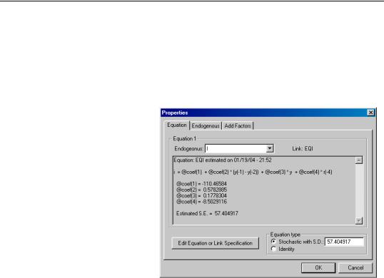
The contents of a line can be examined in more detail using the equation properties dialog. Simply select the line with the mouse, then choose Properties… from the right mouse button menu. Alternatively, simply double click on the object to call up the dialog.

For a link to a single equation, the dialog shows the functional form of the equation, the values of any estimated coefficients, and the standard error of the equation residual from the estimation. If the link is to an object containing many equations, you can move between the different equations imported from the object using the Endogenous list box at the top of the dialog. For an inline equation, the dialog simply shows the text of the equation.

The Edit Equation or Link Specification button allows you to edit the text of an inline equation or to modify a link to point to an object with a different name. A link is represented in text form as a colon followed by the name of the object. Note that you cannot modify the specification of a linked object from within the model object, you must work directly with the linked object itself.

In the bottom right of the dialog, there are a set of fields that allow you to set the stochastic properties of the residual of the equation. If you are only performing deterministic simulations, then these settings will not affect your results in any way. If you are performing stochastic simulations, then these settings are used in conjunction with the solution options to determine the size of the random innovations applied to this equation.

The Stochastic with S.D. option for Equation type lets you set a standard deviation for any random innovations applied to the equation. If the standard deviation field is blank or is set to “NA”, then the standard deviation will be estimated from the historical data. The Identity option specifies that the selected equation is an identity, and should hold without error even in a stochastic simulation. See “Stochastic Options” on page 810 below for further details.

798—Chapter 26. Models

The equation properties dialog also gives you access to the property dialogs for the endogenous variable and add factor associated with the equation. Simply click on the appropriate tab. These will be discussed in greater detail below.

Variable View

The variable view is used for adjusting options related to variables and for displaying and editing the series associated with the model (see the discussion in “An Example Model” (p. 784)). The variable view lists all the variables contained in the model, with each line representing one variable. Each line begins with an icon classifying the variable as endogenous, exogenous or an add factor. This is followed by the name of the variable, the equation number associated with the variable, and the description of the variable. The description is read from the associated series in the workfile.

Note that the names and types of the variables in the model are determined fully by the equations of the model. The only way to add a variable or to change the type of a variable in the model is to modify the model equations.

You can adjust what is displayed in the variable view in a number of ways. By clicking on the Filter/Sort button just above the variable list, you can choose to display only variables that match a certain name pattern, or to display the variables in a particular order. For example, sorting by type of variable makes the division into endogenous and exogenous variables clearer, while sorting by override highlights which variables have been overridden in the currently active scenario.

The variable view also allows you to browse through the dependencies between variables in the model by clicking on the Dependencies button. Each equation in the model can be thought of as a set of links that connect other variables in the model to the endogenous variable of the equation. Starting from any variable, we can travel up the links, showing all the endogenous variables that this variable directly feeds into, or we can travel down the links, showing all the variables upon which this variable directly depends. This may sometimes be useful when trying to find the cause of unexpected behavior. Note, however, that in a simultaneous model, every endogenous variable is indirectly connected to every other variable in the same block, so that it may be hard to understand the model as a whole by looking at any particular part.

You can quickly view or edit one or more of the series associated with a variable by double clicking on the variable. For several variables, simply select each of them with the mouse then double click inside the selected area.

Block Structure View

The block structure view of the model analyzes and displays any block structure in the dependencies of the model.

Working with the Model Structure—799

Block structure refers to whether the model can be split into a number of smaller parts, each of which can be solved for in sequence. For example, consider the system:

block 1

x = y + 4


y = 2*x – 3


block 2

z = x + y


Because the variable Z does not appear in either of the first two equations, we can split this equation system into two blocks: a block containing the first two equations, and a block containing the third equation. We can use the first block to solve for the variables X and Y, then use the second block to solve for the variable Z. By using the block structure of the system, we can reduce the number of variables we must solve for at any one time. This typically improves performance when calculating solutions.

Blocks can be classified further into recursive and simultaneous blocks. A recursive block is one which can be written so that each equation contains only variables whose values have already been determined. A recursive block can be solved by a single evaluation of all the equations in the block. A simultaneous block cannot be written in a way that removes feedback between the variables, so it must be solved as a simultaneous system. In our example above, the first block is simultaneous, since X and Y must be solved for jointly, while the second block is recursive, since Z depends only on X and Y, which have already been determined in solving the first block.

The block structure view displays the structure of the model, labeling each of the blocks as recursive or simultaneous. EViews uses this block structure whenever the model is solved. The block structure of a model may also be interesting in its own right, since reducing the system to a set of smaller blocks can make the dependencies in the system easier to understand.

Text View

The text view of a model allows you to see the entire structure of the model in a single screen of text. This provides a quick way to input small models, or a way to edit larger models using copy-and-paste.

The text view consists of a series of lines. In a simple model, each line simply contains the text of one of the inline equations of the model. More complicated models may contain one of more of the following:

A line beginning with a colon “:” represents a link to an external object. The colon must be followed by the name of an object in the workfile. Equations contained in the external object will be imported into the model whenever the model is opened, or when links are updated.

Соседние файлы в папке Docs