This chapter describes the views and procedures of a group object. With a group, you can compute various statistics that describe the relationship between multiple series and display them in various forms such as spreadsheets, tables, and graphs.
The remainder of this chapter assumes that you are already familiar with the basics of creating and working with a group. See the documentation of EViews features beginning with Chapter 4, “Object Basics”, on page 73 for relevant details on the basic operations.
Group Views Overview
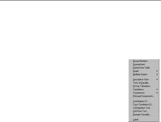
The group view menu is divided into four blocks:
•The views in the first block provide various ways of looking at the actual data in the group.
•The views in the second block display various basics statistics.
•The views in the third block are for specialized statistics typically computed using time series data.
•The fourth block contains the label view, which provides information regarding the group object.
Group Members
This view displays the member series in the group and allows you to alter the group. To change the group, simply edit the group window. You can add other series from the workfile, include expressions involving series, or you can delete series from the group.
Note that editing the window does not change the list of group members. Once you make your changes to the list, you must press the UpdateGroup button in the group window toolbar to save the changes.
Spreadsheet
This view displays the data, in spreadsheet form, for each series in the group. If you wish, you can flip the rows and columns of the spreadsheet by pressing the Transpose button. In transpose format, each row contains a series, and each column an observation or date.
Pressing the Transpose button toggles between the two spreadsheet views.
364—Chapter 12. Groups
You may change the display mode of your spreadsheet view to show various common transformations of your data using the dropdown menu in the group toolbar. By default, EViews displays the original or mapped values in the series using the formatting specified in the series (Default). If you wish, you can change the spreadsheet display to show any transformations defined in the individual series (Series Spec), the underlying series data (Raw Data),
or various differences of the series (in levels or percent changes), with or without log transformations.
You may edit the series data in either levels or transformed values. The Edit +/- on the group toolbar toggles the edit mode for the group. If you are in edit mode, an edit window appears in the top of the group window and a double-box is used to indicate the cell that is being edited.
Here, we are editing the data in the group in 1-period percent changes (note the label to the right of the edit field). If we change the 1952Q4 value of the percent change in GDP,
from 3.626 to 5, the values of GDP from 1952Q4 to the end of the workfile will change to reflect the one-time increase in the value of GDP.
EViews provides you with additional tools for altering the display of your spreadsheet. To change the display properties, select one or more series by clicking on the series names in the headers, then right-click to bring up a menu.
If you right-click and then select Display format... EViews will open a format dialog that will allow you to override the individual series display characteristics. Once you specify the desired format and click on OK, EViews will update the group display to reflect your specification.
Note that, by default, changes to the group display format will apply only to the group spreadsheet and will not change the underlying series characteristics. If, for example, you elect to show series X in fixed decimal format in the group spreadsheet, but X uses significant digits in its individual series settings, the latter settings will not be modified. To update the display settings in the selected series, you must select the Apply to underlying series checkbox in the format dialog.
Dated Data Table—365
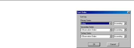
Most of the other right-mouse menu items should be self-explanatory. Note that you may choose to sort the observations in the group by selecting Sort.... EViews will open the Sort Order dialog, prompting you to select sort keys and orders for up to three series.
When you click on OK, EViews will rearrange the group spreadsheet display so that observations are displayed in the specified order.
Note that the underlying data in the workfile
is not sorted, only the display of observations and observation identifiers in the group spreadsheet. This method of changing the spreadsheet display may prove useful if you wish to determine the identities of observations with high or low values for some series in the group.
Lastly, you should note that as with series, you may write the contents of the spreadsheet view to a CSV, tab-delimited ASCII text, RTF, or HTML file by selecting Save table to disk... and filling out the resulting dialog.
Dated Data Table
The dated data table view is used to construct tables for reporting and presenting data, forecasts, and simulation results. This view displays the series contained in the group in a variety of formats. You can also use this view to perform common transformations and frequency conversions, and to display data at various frequencies in the same table.
For example, suppose you wish to show your quarterly data for the GDP and PR series, with data for each year, along with an annual average, on a separate line:
1994
1994
GDP
1698.6
1727.9
1746.7
1774.0
1736.8
PR
1.04
1.05
1.05
1.06
1.05
1995
1995
GDP
1792.3
1802.4
1825.3
1845.5
1816.4
PR
1.07
1.07
1.08
1.09
1.08
1996
1996
GDP
1866.9
1902.0
1919.1
1948.2
1909.0
PR
1.09
1.10
1.11
1.11
1.10
The dated data table handles all of the work of setting up this table, and computing the summary values.
366—Chapter 12. Groups
Alternatively, you may wish to display annual averages for each year up to the last, followed by the last four quarterly observations in your sample:
1994
1995
1996
96:1
96:2
96:3
96:4
GDP
1736.8
1816.4
1909.0
1866.9
1902.0
1919.1
1948.2
PR
1.05
1.08
1.10
1.09
1.10
1.11
1.11
Again, the dated data table may be used to perform the required calculations and to set up the table automatically.
The dated data table is capable of creating more complex tables and performing a variety of other calculations. Note, however, that the dated data table view is currently available only for annual, semi-annual, quarterly, or monthly workfiles.
Creating and Specifying a Dated Data Table
To create a dated data table, create a group containing the series of interest and select View/Dated Data Table. The group window initially displays a default table view. The default is to show a single year of data on each line, along with a summary measure (the annual average).
You can, however, set options to control the display of your data through the Table and Row Options dialogs. Note the presence of two new buttons on the group window toolbar, labeled TabOptions (for Table Options) and RowOptions. TabOptions sets the global options for the dated data table. These options will apply to all series in the group object. The RowOptions button allows you to override the global options for a particular series. Once you specify table and row options for your group, EViews will remember these options the next time you open the dated data table view for the group.
Table Setup
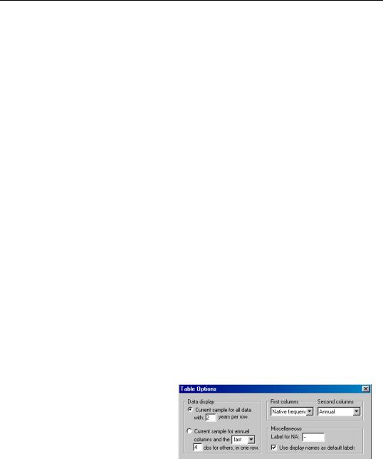
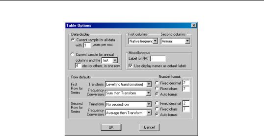
When you click on the TabOptions button, the Table Options dialog appears. The top half of the dialog provides options to control the general style of the table.
The radio buttons on the left hand side of the dialog allow you to choose between the two display formats described above:
•The first style displays the data for n years per row, where n is the positive integer specified in the edit field.
•The second style is a bit more complex. It allows you to specify, for data displayed at a frequency other than annual, the number of observations taken from the end of the
Dated Data Table—367
workfile sample that are to be displayed. For data displayed at an annual frequency, EViews will display observations over the entire workfile sample.
The two combo boxes on the top right of the dialog supplement your dated display choice by allowing you to display your data at multiple frequencies in each row. The First Columns selection describes the display frequency for the first group of columns, while the Second Columns selection controls the display for the second group of columns. If you select the same frequency, only one set of results will be displayed.
In each combo box, you may choose among:
•Native frequency (the frequency of the workfile)
•Annual
•Quarterly
•Monthly
If necessary, EViews will perform any frequency conversion (to a lower frequency) required to construct the table.
The effects of these choices on the table display are best described by the following example. For purposes of illustration, note that the current workfile is quarterly, with a current sample of 1993Q1–1996Q4.
Now suppose that you choose to display the first style (two years per row), with the first columns set to the native frequency, and the second columns set to annual frequency. Each row will contain eight quarters of data (the native frequency data) followed by the corresponding two annual observations (the annual frequency data):
Q1
Q2
Q3
Q4
Q1
Q2
Q3
Q4
Year
1993
1994
1993
1994
GDP
1611.1
1627.3
1643.6
1676.0
1698.6
1727.9
1746.7
1774.0
1639.5
1736.8
PR
1.02
1.02
1.03
1.04
1.04
1.05
1.05
1.06
1.03
1.05
1995
1996
1995
1996
GDP
1792.3
1802.4
1825.3
1845.5
1866.9
1902.0
1919.1
1948.2
1816.4
1909.0
PR
1.07
1.07
1.08
1.09
1.09
1.10
1.11
1.11
1.08
1.10
EViews automatically performs the frequency conversion to annual data using the specified method (see “Transformation Methods” on page 368).
If you reverse the ordering of data types in the first and second columns so that the first columns display the annual data, and the second columns display the native frequency, the dated data table will contain:
368—Chapter 12. Groups
Q1
Q2
Q3
Q4
Q1
Q2
Q3
Q4
1993
1994
1993
1994
GDP
1639.5
1736.8
1611.1
1627.3
1643.6
1676.0
1698.6
1727.9
1746.7
1774.0
PR
1.03
1.05
1.02
1.02
1.03
1.04
1.04
1.05
1.05
1.06
1995
1996
1995
1996
GDP
1816.4
1909.0
1792.3
1802.4
1825.3
1845.5
1866.9
1902.0
1919.1
1948.2
PR
1.08
1.10
1.07
1.07
1.08
1.09
1.09
1.10
1.11
1.11
Now, click on TabOptions, choose the second display style, and enter 4 in the edit box. Then specify Annual frequency for the first columns and Native frequency for the second columns. EViews will display the annual data for the current sample, followed by the last four quarterly observations:
1993
1994
1995
1996
96:1
96:2
96:3
96:4
GDP
1639.5
1736.8
1816.4
1909.0
1866.9
1902.0
1919.1
1948.2
PR
1.03
1.05
1.08
1.10
1.09
1.10
1.11
1.11
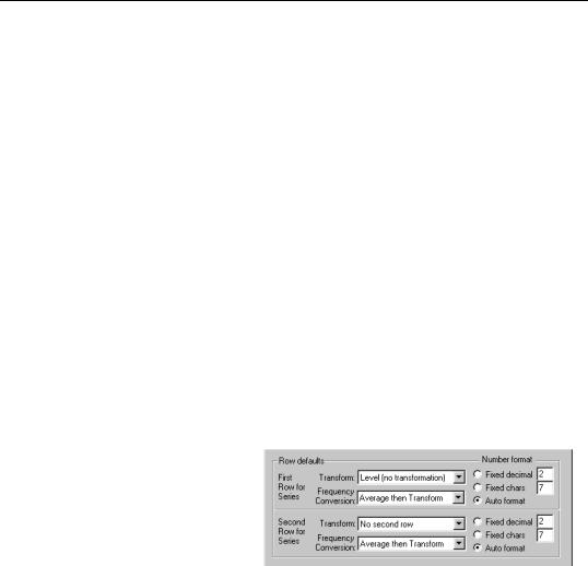
Additional Table Options
The bottom of the Table Options dialog controls the default data transformations and numeric display for each series in the group. EViews allows you to use two rows, each with a different transformation and a different output format, to describe each series.
For each row, you specify the transformation method, frequency conversion method, and the number format.
Keep in mind that you may override the default transformation for a particular series using the RowOptions menu (p. 371).
Transformation Methods
The following transformations are available:
None (raw data)
No transformation
1 Period Difference
( y − y( −1 ) )
Dated Data Table—369
1
Year Difference
1
for annual
2
for semi-annual
y − y( −f) , wheref =
4
for quarterly
12 for monthly
1
Period % Change
100 × ( y − y( −1) ) ⁄ y( −1)
1
Period % Change at
Computes R such that:
Annual Rate
( 1 + r
⁄ 100 )f
where f is defined above and r is the 1 period%
change.
1
Year % Change
100 × ( y − y( −f) ) ⁄ y( −f) , where f is defined
above.
No second row
Do not display a second row
We emphasize that the above transformation methods represent only the most commonly employed transformations. If you wish to construct your table with other transformations, you should add an appropriate auto-series to the group.
Frequency Conversion
The following frequency conversion methods are provided:
Average then Trans-
First convert by taking the average, then trans-
form
form the average, as specified.
Transform then Aver-
First transform the series, then take the aver-
age
age of the transformed series.
Sum then Transform
First convert by taking the sum, then trans-
form the sum, as specified.
First Period
Convert by taking the first quarter of each year
or first month of each quarter/year.
Last Period
Convert by taking the last quarter of each year
or last month of each quarter/year.
The choice between Average then Transform and Transform then Average changes the ordering of the transformation and frequency conversion operations. The methods differ only for nonlinear transformations (such as the % change methods).
For example, if we specify the dated data table settings:
370—Chapter 12. Groups
EViews will display a table with data formatted in the following fashion:
Q1
Q2
Q3
Q4
Year
1993
1993
GDP
1611.1
1627.3
1643.6
1676.0
6558.1
PR
1.02
1.02
1.03
1.04
4.11
1994
1994
GDP
1698.6
1727.9
1746.7
1774.0
6947.1
PR
1.04
1.05
1.05
1.06
4.20
1995
1995
GDP
1792.3
1802.4
1825.3
1845.5
7265.4
PR
1.07
1.07
1.08
1.09
4.31
1996
1996
GDP
1866.9
1902.0
1919.1
1948.2
7636.1
PR
1.09
1.10
1.11
1.11
4.41
If, instead, you change the Frequency Conversion to First Period, EViews will display a table of the form:
Dated Data Table—371
Q1
Q2
Q3
Q4
Year
1993
1993
GDP
1611.1
1627.3
1643.6
1676.0
1611.1
PR
1.02
1.02
1.03
1.04
1.02
1994
1994
GDP
1698.6
1727.9
1746.7
1774.0
1698.6
PR
1.04
1.05
1.05
1.06
1.04
1995
1995
GDP
1792.3
1802.4
1825.3
1845.5
1792.3
PR
1.07
1.07
1.08
1.09
1.07
1996
1996
GDP
1866.9
1902.0
1919.1
1948.2
1866.9
PR
1.09
1.10
1.11
1.11
1.09
In “Illustration” beginning on page 372, we provide an example which illustrates the computation of the percentage change measures.
Formatting Options
EViews lets you choose between fixed decimal, fixed digit, and auto formatting of the numeric data. Generally, auto formatting will produce appropriate output formatting, but if not, simply select the desired method and enter an integer in the edit field. The options are:
Auto format EViews chooses the format depending on the data.
Fixed decimal Specify how many digits to display after the decimal point. This option aligns all numbers at the decimal point.
Fixed chars Specify how many total characters to display for each number.
EViews will round your data prior to display in order to fit the specified format. This rounding is for display purposes only and does not alter the original data.
Row Options
These options allow you to override the row defaults specified by the Table Options dialog. You can specify a different transformation, frequency conversion method, and number format, for each series.
372—Chapter 12. Groups
In the Series Table Row Description dialog that appears, select the series for which you wish to override the table default options. Then specify the transformation, frequency conversion, or number format you want to use for that series. The options are the same as those described above for the row defaults.
Other Options
Label for NA: allows you to define the symbol used to identify missing values in the table. Bear in mind that if you choose to display
your data in transformed form, the transformation may generate missing values even if none of the raw data are missing. Dated data table transformations are explained above.
If your series has display names, you can use the display name as the label for the series in the table by selecting the Use display names as default labels option. See Chapter 3 for a discussion of display names and the label view.
Illustration
As an example, consider the following dated data table which displays both quarterly and annual data for GDP and PR in 1995 and 1996:
1995
1995
GDP
1792.3
1802.4
1825.3
1845.5
1816.4
(% ch.)
1.03
0.56
1.27
1.11
4.58
PR
1.07
1.07
1.08
1.09
1.08
(% ch.)
0.80
0.49
0.52
0.55
2.55
1996
1996
GDP
1866.9
1902.0
1919.1
1948.2
1909.0
(% ch.)
1.16
1.88
0.90
1.52
5.10
PR
1.09
1.10
1.11
1.11
1.10
(% ch.)
0.72
0.41
0.64
0.46
2.27
At the table level, the first row of output for each of the series is set to be untransformed, while the second row will show the 1-period percentage change in the series. The table defaults have both rows set to perform frequency conversion using the Average then
Dated Data Table—373
Transformed setting. In addition, we use Series Table Row Options dialog to override the second row transformation for PR, setting it to Transform then Average option.
The first four columns show the data in native frequency so the choice between Average then Transform and Transform then Average is irrelevant—each entry in the second row measures the 1-period (1-quarter) percentage change in the variable.
The 1-period percentage change in the last column is computed differently under the two methods. The Average then Transformed percentage change in GDP for 1996 measures the percentage change between the average value in 1995 and the average value in 1996. It is computed as:
100 ( 1909.0 − 1816.3 ) ⁄ 1816.4 5.10
(12.1)
EViews computes this transformation using full precision for intermediate results, then displays the result using the specified number format.
The computation of the Transform then Average one-period change in PR for 1996 is a bit more subtle. Since we wish to compute measure of the annual change, we first evaluate the one-year percentage change at each of the quarters in the year, and then average the results. For example, the one-year percentage change in 1996Q1 is given by 100(1.09-1.03)/ 1.03=2.29 and the one-year percentage change in 1996Q2 is 100(1.10-1.07)/1.07=2.22. Averaging these percentage changes yields:
100
1.09 − 1.07
+
1.10 − 1.07
+
1.11 − 1.08
+
1.11 − 1.09
⁄ 4 2.27 (12.2)
--------------------------1.07-
--------------------------1.07-
--------------------------1.08-
--------------------------1.09-
Note also that this computation differs from evaluating the average of the one-quarter percentage changes for each of the quarters of the year.
Other Menu Items
•Edit+/– allows you to edit the row (series) labels as well as the actual data in the table. You will not be able to edit any of the computed ranks and any changes that you make to the row labels will only apply to the dated data table view.
We warn you that if you edit a data cell, the underlying series data will also change. This latter feature allows you to use dated data tables for data entry from published sources.
If you want to edit the data in the table but wish to keep the underlying data unchanged, first Freeze the table view and then apply Edit to the frozen table.
•Font allows you to choose the font, font style, and font size to be used in the table.
•Title allows you to add a title to the table.
•Sample allows you to change the sample to display in the table.