Two-stage Least Squares—473

HAC Consistent Covariances (Newey-West)

The White covariance matrix described above assumes that the residuals of the estimated equation are serially uncorrelated. Newey and West (1987) have proposed a more general covariance estimator that is consistent in the presence of both heteroskedasticity and autocorrelation of unknown form. The Newey-West estimator is given by,

and q , the truncation lag, is a parameter representing the number of autocorrelations used in evaluating the dynamics of the OLS residuals ut . Following the suggestion of Newey and West, EViews sets q using the formula:

To use the Newey-West method, select the Options tab in the Equation Estimation. Check the box labeled Heteroskedasticity Consistent Covariance and press the Newey-West radio button.

Two-stage Least Squares

A fundamental assumption of regression analysis is that the right-hand side variables are uncorrelated with the disturbance term. If this assumption is violated, both OLS and weighted LS are biased and inconsistent.

There are a number of situations where some of the right-hand side variables are correlated with disturbances. Some classic examples occur when:

•There are endogenously determined variables on the right-hand side of the equation.

•Right-hand side variables are measured with error.

For simplicity, we will refer to variables that are correlated with the residuals as endogenous, and variables that are not correlated with the residuals as exogenous or predetermined.

The standard approach in cases where right-hand side variables are correlated with the residuals is to estimate the equation using instrumental variables regression. The idea

474—Chapter 16. Additional Regression Methods

behind instrumental variables is to find a set of variables, termed instruments, that are both (1) correlated with the explanatory variables in the equation, and (2) uncorrelated with the disturbances. These instruments are used to eliminate the correlation between right-hand side variables and the disturbances.

Two-stage least squares (TSLS) is a special case of instrumental variables regression. As the name suggests, there are two distinct stages in two-stage least squares. In the first stage, TSLS finds the portions of the endogenous and exogenous variables that can be attributed to the instruments. This stage involves estimating an OLS regression of each variable in the model on the set of instruments. The second stage is a regression of the original equation, with all of the variables replaced by the fitted values from the first-stage regressions. The coefficients of this regression are the TSLS estimates.

You need not worry about the separate stages of TSLS since EViews will estimate both stages simultaneously using instrumental variables techniques. More formally, let Z be the matrix of instruments, and let y and X be the dependent and explanatory variables. Then the coefficients computed in two-stage least squares are given by,

and the estimated covariance matrix of these coefficients is given by:

where s2 is the estimated residual variance (square of the standard error of the regression).

Estimating TSLS in EViews

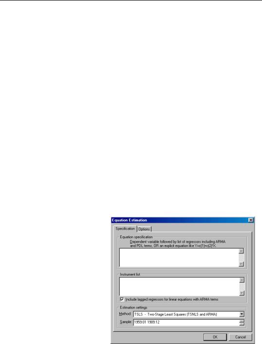
To use two-stage least squares, open the equation specification box by choosing Object/New Object.../Equation… or Quick/Estimate Equation…. Choose TSLS from the Method: combo box and the dialog will change to include an edit window where you will list the instruments.

In the Equation specification edit box, specify your dependent variable and independent variables, and in the Instrument list edit box, provide a list of instruments.

Two-stage Least Squares—475

There are a few things to keep in mind as you enter your instruments:

•In order to calculate TSLS estimates, your specification must satisfy the order condition for identification, which says that there must be at least as many instruments as there are coefficients in your equation. There is an additional rank condition which must also be satisfied. See Davidson and MacKinnon (1994) and Johnston and DiNardo (1997) for additional discussion.

•For econometric reasons that we will not pursue here, any right-hand side variables that are not correlated with the disturbances should be included as instruments.

•The constant, C, is always a suitable instrument, so EViews will add it to the instrument list if you omit it.

For example, suppose you are interested in estimating a consumption equation relating consumption (CONS) to gross domestic product (GDP), lagged consumption (CONS(–1)), a trend variable (TIME) and a constant (C). GDP is endogenous and therefore correlated with the residuals. You may, however, believe that government expenditures (G), the log of the money supply (LM), lagged consumption, TIME, and C, are exogenous and uncorrelated with the disturbances, so that these variables may be used as instruments. Your equation specification is then,

cons c gdp cons(-1) time

and the instrument list is:

c gov cons(-1) time lm

This specification satisfies the order condition for identification, which requires that there are at least as many instruments (five) as there are coefficients (four) in the equation specification.

Furthermore, all of the variables in the consumption equation that are believed to be uncorrelated with the disturbances, (CONS(–1), TIME, and C), appear both in the equation specification and in the instrument list. Note that listing C as an instrument is redundant, since EViews automatically adds it to the instrument list.

Output from TSLS

Below, we present TSLS estimates from a regression of LOG(CS) on a constant and LOG(GDP), with the instrument list “C LOG(CS(-1)) LOG(GDP(-1))”:

476—Chapter 16. Additional Regression Methods

Dependent Variable: LOG(CS)

Method: Two-Stage Least Squares

Date: 10/15/97 Time: 11:32

Sample(adjusted): 1947:2 1995:1

Included observations: 192 after adjusting endpoints

Instrument list: C LOG(CS(-1)) LOG(GDP(-1))

EViews identifies the estimation procedure, as well as the list of instruments in the header. This information is followed by the usual coefficient, t-statistics, and asymptotic p-values.

The summary statistics reported at the bottom of the table are computed using the formulas outlined in “Summary Statistics” on page 451. Bear in mind that all reported statistics are only asymptotically valid. For a discussion of the finite sample properties of TSLS, see Johnston and DiNardo (1997, pp. 355–358) or Davidson and MacKinnon (1984, pp. 221– 224).

EViews uses the structural residuals ut = yt − xt′bTSLS in calculating all of the summary statistics. For example, the standard error of the regression used in the asymptotic

covariance calculation is computed as:

These structural residuals should be distinguished from the second stage residuals that you would obtain from the second stage regression if you actually computed the two-stage least squares estimates in two separate stages. The second stage residuals are given by

sions.

We caution you that some of the reported statistics should be interpreted with care. For example, since different equation specifications will have different instrument lists, the reported R2 for TSLS can be negative even when there is a constant in the equation.

Weighted TSLS

You can combine TSLS with weighted regression. Simply enter your TSLS specification as above, then press the Options button, select the Weighted LS/TSLS option, and enter the weighting series.

Two-stage Least Squares—477

Weighted two-stage least squares is performed by multiplying all of the data, including the instruments, by the weight variable, and estimating TSLS on the transformed model. Equivalently, EViews then estimates the coefficients using the formula,

TSLS with AR errors

You can adjust your TSLS estimates to account for serial correlation by adding AR terms to your equation specification. EViews will automatically transform the model to a nonlinear least squares problem, and estimate the model using instrumental variables. Details of this procedure may be found in Fair (1984, pp. 210–214). The output from TSLS with an AR(1) specification looks as follows:

Dependent Variable: LOG(CS)

Method: Two-Stage Least Squares

Date: 10/15/97 Time: 11:42

Sample(adjusted): 1947:2 1995:1

Included observations: 192 after adjusting endpoints

Convergence achieved after 4 iterations

Instrument list: C LOG(CS(-1)) LOG(GDP(-1))

The Options button in the estimation box may be used to change the iteration limit and convergence criterion for the nonlinear instrumental variables procedure.

First-order AR errors

Suppose your specification is:

yt = xt′β + wtγ + ut

(16.22)

ut = ρ1ut − 1 + t

478—Chapter 16. Additional Regression Methods

where xt is a vector of endogenous variables, and wt is a vector of predetermined variables, which, in this context, may include lags of the dependent variable. zt is a vector of instrumental variables not in wt that is large enough to identify the parameters of the model.

In this setting, there are important technical issues to be raised in connection with the choice of instruments. In a widely quoted result, Fair (1970) shows that if the model is estimated using an iterative Cochrane-Orcutt procedure, all of the lagged leftand right-hand side variables (yt − 1, xt − 1, wt − 1) must be included in the instrument list to obtain consistent estimates. In this case, then the instrument list should include:

Despite the fact the EViews estimates the model as a nonlinear regression model, the first stage instruments in TSLS are formed as if running Cochrane-Orcutt. Thus, if you choose to omit the lagged leftand right-hand side terms from the instrument list, EViews will automatically add each of the lagged terms as instruments. This fact is noted in your output.

Higher Order AR errors

The AR(1) result extends naturally to specifications involving higher order serial correlation. For example, if you include a single AR(4) term in your model, the natural instrument list will be:

Note that while theoretically valid, this instrument list has a large number of overidentifying instruments, which may lead to computational difficulties and large finite sample biases (Fair (1984, p. 214), Davidson and MacKinnon (1993, pp. 222-224)). In theory, adding instruments should always improve your estimates, but as a practical matter this may not be so in small samples.

Examples

Suppose that you wish to estimate the consumption function by two-stage least squares, allowing for first-order serial correlation. You may then use two-stage least squares with the variable list,

cons c gdp ar(1)

and instrument list:

Two-stage Least Squares—479

c gov log(m1) time cons(-1) gdp(-1)

Notice that the lags of both the dependent and endogenous variables (CONS(–1) and GDP(–1)), are included in the instrument list.

Similarly, consider the consumption function:

cons c cons(-1) gdp ar(1)

A valid instrument list is given by:

c gov log(m1) time cons(-1) cons(-2) gdp(-1)

Here we treat the lagged left and right-hand side variables from the original specification as predetermined and add the lagged values to the instrument list.

Lastly, consider the specification:

cons c gdp ar(1) ar(2) ar(3) ar(4)

Adding all of the relevant instruments in the list, we have:

c gov log(m1) time cons(-1) cons(-2) cons(-3) cons(-4) gdp(-1) gdp(-2) gdp(-3) gdp(-4)

TSLS with MA errors

You can also estimate two-stage least squares variable problems with MA error terms of various orders. To account for the presence of MA errors, simply add the appropriate terms to your specification prior to estimation.

Illustration

Suppose that you wish to estimate the consumption function by two-stage least squares, accounting for first-order moving average errors. You may then use two-stage least squares with the variable list,

cons c gdp ma(1)

and instrument list:

c gov log(m1) time

EViews will add both first and second lags of CONS and GDP to the instrument list.

Technical Details

Most of the technical details are identical to those outlined above for AR errors. EViews transforms the model that is nonlinear in parameters (employing backcasting, if appropriate) and then estimates the model using nonlinear instrumental variables techniques.