Добавил:
Upload Опубликованный материал нарушает ваши авторские права? Сообщите нам.
Вуз: Предмет: Файл:
Eviews5 / EViews5 / Docs / EViews 5 Users Guide.pdf
Скачиваний:
152
Добавлен:
23.03.2015
Размер:
11.51 Mб
Скачать

908—Chapter 29. Panel Estimation

“@LEV” is not provided, EViews will transform the instrument to match the equation transformation.

If, for example, you estimate an equation that uses orthogonal deviations to remove a cross-section fixed effect, EViews will, by default, compute orthogonal deviations of the instruments provided prior to their use. Thus, the instrument list:

z1 z2 @lev(z3)

will use the transformed Z1 and Z2, and the original Z3 as the instruments for the specification.

Note that in specifications where “@DYN” and “@LEV” keywords are not relevant, they will be ignored. If, for example, you first estimate a GMM specification using first differences with both dynamic and level instruments, and then re-estimate the equation using LS, EViews will ignore the keywords, and use the instruments in their original forms.

GMM Options

Lastly, clicking on the Options tab in the dialog brings up a page displaying computational options for GMM estimation. These options are virtually identical to those for both LS and IV estimation (see “LS Options” on page 904). The one difference is in the option for saving estimation weights with the object. In the GMM context, this option applies to both the saving of GLS as well as GMM weights.

Panel Estimation Examples

Least Squares Examples

To illustrate the estimation of panel equations in EViews, we first consider an example involving unbalanced panel data from Harrison and Rubinfeld (1978) for the study of hedonic pricing. The data are well known and used as an example dataset in many sources (e.g., Baltagi (2001), p. 166).

The data consist of 506 census tract observations on 92 towns in the Boston area with group sizes ranging from 1 to 30. The dependent variable of interest is the median value of owner occupied towns (MV), and the regressors include various measures of housing desirability.

We begin our example by structuring our workfile as an undated panel. Click on the “Range:” description in the workfile window,

Panel Estimation Examples—909

select Undated Panel, and enter “TOWNID” as the Identifier series. EViews will prompt you twice to create a CELLID series to uniquely identify observations. Click on OK to both questions to accept your settings.

EViews restructures your workfile so that it is an unbalanced panel workfile. The top portion of the workfile window will change to show the undated structure which has 92 cross-sections and a maximum of 30 observations in a cross-section.

Next, we open the equation specification dialog by selecting Quick/Estimate Equation from the main EViews menu.

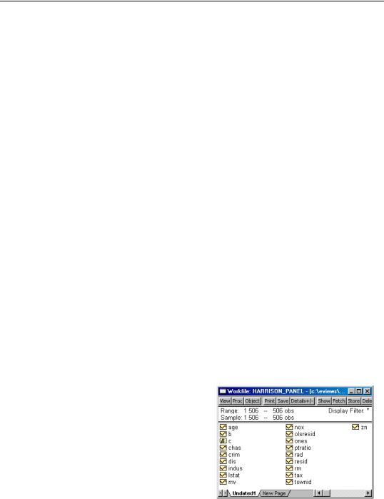
First, following Baltagi and Chang (1994) (also described in Baltagi, 2001), we estimate a fixed effects specification of a hedonic housing equation. The dependent variable in our specification is the median value MV, and the regressors are the crime rate (CRIM), a

dummy variable for the property along Charles River (CHAS), air pollution (NOX), average number of rooms (RM), proportion of older units (AGE), distance from employment centers (DIS), proportion of African-Americans in the population (B), and the proportion of lower status individuals (LSTAT). Note that you may include a constant term C in the specification. Since we are estimating a fixed effects specification, EViews will add one if it is not present so that the fixed effects estimates are relative to the constant term and add up to zero.

Click on the Panel Options tab and select Fixed for the Cross-section effects. To match the Baltagi and Chang results, we will leave the remaining settings at their defaults. Click on OK to accept the specification.

910—Chapter 29. Panel Estimation

Dependent Variable: MV

Method: Panel Least Squares

Date: 02/16/04 Time: 12:07

Sample: 1 506

Cross-sections included: 92

Total panel (unbalanced) observations: 506

Variable

Coefficient

Std. Error

t-Statistic

Prob.


C

8.993272

0.134738

66.74632

0.0000

CRIM

-0.625400

0.104012

-6.012746

0.0000

CHAS

-0.452414

0.298531

-1.515467

0.1304

NOX

-0.558938

0.135011

-4.139949

0.0000

RM

0.927201

0.122470

7.570833

0.0000

AGE

-1.406955

0.486034

-2.894767

0.0040

DIS

0.801437

0.711727

1.126045

0.2608

B

0.663405

0.103222

6.426958

0.0000

LSTAT

-2.453027

0.255633

-9.595892

0.0000


Effects Specification

Cross-section fixed (dummy variables)

R-squared

0.918370

Mean dependent var

9.942268

Adjusted R-squared

0.898465

S.D. dependent var

0.408758

S.E. of regression

0.130249

Akaike info criterion

-1.063668

Sum squared resid

6.887683

Schwarz criterion

-0.228384

Log likelihood

369.1080

F-statistic

46.13805

Durbin-Watson stat

1.999986

Prob(F-statistic)

0.000000


The results for the fixed effects estimation are depicted here. Note that as in pooled estimation, the reported R-squared and F-statistics are based on the difference between the residuals sums of squares from the estimated model, and the sums of squares from a single constant-only specification, not from a fixed-effect-only specification. Similarly, the reported information criteria report likelihoods adjusted for the number of estimated coefficients, including fixed effects. Lastly, the reported Durbin-Watson stat is formed simply by computing the first-order residual correlation on the stacked set of residuals.

We may click on the Estimate button to modify the specification to match the WallaceHussain random effects specification considered by Baltagi and Chang. We modify the specification to include the additional regressors used in estimation, change the cross-sec- tion effects to be estimated as a random effect, and use the Options page to set the random effects computation method to Wallace-Hussain.

The top portion of the resulting output is given by:

Panel Estimation Examples—911

Dependent Variable: MV

Method: Panel EGLS (Cross-section random effects)

Date: 02/16/04 Time: 12:28

Sample: 1 506

Cross-sections included: 92

Total panel (unbalanced) observations: 506

Wallace and Hussain estimator of component variances

Variable

Coefficient

Std. Error

t-Statistic

Prob.


C

9.684427

0.207691

46.62904

0.0000

CRIM

-0.737616

0.108966

-6.769233

0.0000

ZN

0.072190

0.684633

0.105443

0.9161

INDUS

0.164948

0.426376

0.386860

0.6990

CHAS

-0.056459

0.304025

-0.185703

0.8528

NOX

-0.584667

0.129825

-4.503496

0.0000

RM

0.908064

0.123724

7.339410

0.0000

AGE

-0.871415

0.487161

-1.788760

0.0743

DIS

-1.423611

0.462761

-3.076343

0.0022

RAD

0.961362

0.280649

3.425493

0.0007

TAX

-0.376874

0.186695

-2.018658

0.0441

PTRATIO

-2.951420

0.958355

-3.079674

0.0022

B

0.565195

0.106121

5.325958

0.0000

LSTAT

-2.899084

0.249300

-11.62891

0.0000


Effects Specification


Cross-section random S.D. / Rho


0.126983

0.4496

Idiosyncratic random S.D. / Rho


0.140499

0.5504


Note that the estimates of the component standard deviations must be squared to match the component variances reported by Baltagi and Chang (0.016 and 0.020, respectively).

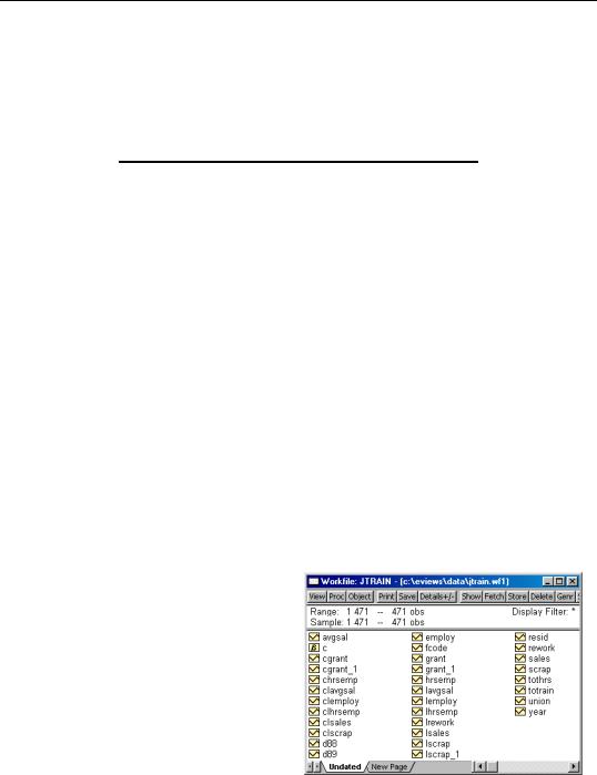
Next, we consider an example of estimation with standard errors that are robust to serial correlation. For this example, we employ data on job training grants used in examples from Wooldridge (2002, p. 276 and 282).

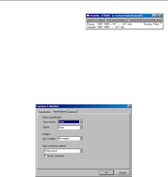
As before, the first step is to structure the workfile as a panel workfile. Click on Range: to bring up the dialog, and enter “YEAR” as the date identifier and “FCODE” as the cross-section ID.

912—Chapter 29. Panel Estimation

EViews will structure the workfile so that it is a panel workfile with 157 cross-sections, and three annual observations. Note that even though there are 471 observations in the workfile, a

large number of them contain missing values for variables of interest.

To estimate the fixed effect specification with robust standard errors (Wooldridge example 10.5, p. 276), click on specification Quick/Estimate Equation from the main EViews menu. Enter the list specification:

lscrap c d88 d89 grant grant_1

in the Equation specification edit box on the main page and select Fixed in the Cross-sec- tion effects specification combo box on the Panel Options page. Lastly, since we wish to compute standard errors that are robust to serial correlation (Arellano (1987), White (1984)), we choose White period as the Coef covariance method. To match the reported Wooldridge example, we must select No d.f. correction in the covariance calculation.

Click on OK to accept the options. EViews displays the results from estimation:

Panel Estimation Examples—913

Dependent Variable: LSCRAP

Method: Panel Least Squares

Date: 02/16/04 Time: 13:28

Sample: 1987 1989

Cross-sections included: 54

Total panel (balanced) observations: 162

White period standard errors & covariance (no d.f. correction)

Variable

Coefficient

Std. Error

t-Statistic

Prob.


C

0.597434

0.062489

9.560565

0.0000

D88

-0.080216

0.095719

-0.838033

0.4039

D89

-0.247203

0.192514

-1.284075

0.2020

GRANT

-0.252315

0.140329

-1.798022

0.0751

GRANT_1

-0.421589

0.276335

-1.525648

0.1301


Effects Specification

Cross-section fixed (dummy variables)

R-squared

0.927572

Mean dependent var

0.393681

Adjusted R-squared

0.887876

S.D. dependent var

1.486471

S.E. of regression

0.497744

Akaike info criterion

1.715383

Sum squared resid

25.76593

Schwarz criterion

2.820819

Log likelihood

-80.94602

F-statistic

23.36680

Durbin-Watson stat

1.996983

Prob(F-statistic)

0.000000


Note that EViews automatically adjusts for the missing values in the data. There are only 162 observations on 54 cross-sections used in estimation. The top portion of the output indicates that the results use robust White period standard errors with no d.f. correction.

Alternately, we may estimate a first difference estimator for these data with robust standard errors (Wooldridge example 10.6, p. 282). Open a new equation dialog by clicking on Quick/Estimate Equation..., or modify the existing equation by clicking on the Estimate button on the equation toolbar. Enter the specification:

d(lscrap) c d89 d(grant) d(grant_1)

in the Equation specification edit box on the main page, select None in the Cross-section effects specification combo box, and White period with No d.f. correction for the coefficient covariance method on the Panel Options page. The reported results are given by:

914—Chapter 29. Panel Estimation

Dependent Variable: D(LSCRAP)

Method: Panel Least Squares

Date: 02/16/04 Time: 14:51

Sample (adjusted): 1988 1988

Cross-sections included: 54

Total panel (balanced) observations: 108

White period standard errors & covariance (d.f. corrected)

Variable

Coefficient

Std. Error

t-Statistic

Prob.


C

-0.090607

0.089760

-1.009442

0.3151

D89

-0.096208

0.113117

-0.850519

0.3970

D(GRANT)

-0.222781

0.131030

-1.700236

0.0921

D(GRANT_1)

-0.351246

0.269704

-1.302339

0.1957


R-squared

0.036518

Mean dependent var

-0.221132

Adjusted R-squared

0.008725

S.D. dependent var

0.579248

S.E. of regression

0.576716

Akaike info criterion

1.773399

Sum squared resid

34.59049

Schwarz criterion

1.872737

Log likelihood

-91.76352

F-statistic

1.313929

Durbin-Watson stat

1.498132

Prob(F-statistic)

0.273884


While current versions of EViews do not provide a full set of specification tests for panel equations, it is a straightforward task to construct some tests using residuals obtained from the panel estimation.

To continue with the Wooldridge example, we may test for AR(1) serial correlation in the first-differenced equation by regressing the residuals from this specification on the lagged residuals using data for the year 1989. First, we save the residual series in the workfile.

Click on Proc/Make Residual Series... on the estimated equation toolbar, and save the residuals to the series RESID01.

Next, regress RESID01 on RESID01(-1), yielding:

Panel Estimation Examples—915

Dependent Variable: RESID01

Method: Panel Least Squares

Date: 02/16/04 Time: 14:57

Sample (adjusted):

Cross-sections included: 54

Total panel (balanced) observations: 54

Variable

Coefficient

Std. Error

t-Statistic

Prob.


RESID01(-1)

0.236906

0.133357

1.776481

0.0814


R-squared

0.056199

Mean dependent var

2.06E-18

Adjusted R-squared

0.056199

S.D. dependent var

0.571061

S.E. of regression

0.554782

Akaike info criterion

1.677863

Sum squared resid

16.31252

Schwarz criterion

1.714696

Log likelihood

-44.30230

Durbin-Watson stat

0.000000


Under the null hypothesis that the original idiosyncratic errors are uncorrelated, the residuals from this equation should have an autocorrelation coefficient of -0.5. Here, we obtain an estimate of ρˆ 1 = 0.237 which appears to be far from the null value. A formal Wald hypothesis test rejects the null that the original idiosyncratic errors are serially uncorrelated:

Wald Test:

Equation: Untitled

Test Statistic

Value

df

Probability


F-statistic

26.60396

(1, 53)

0.0000

Chi-square

26.60396

1

0.0000


Null Hypothesis Summary:


Normalized Restriction (= 0)

Value

Std. Err.


0.5 + C(1)


0.736906

0.142869


Restrictions are linear in coefficients.

Instrumental Variables Example

To illustrate the estimation of instrumental variables panel estimators, we consider an example taken from Papke (1994) for enterprise zone data for 22 communities in Indiana that is outlined in Wooldridge (2002, p. 306).

916—Chapter 29. Panel Estimation

The panel workfile for this example is structured using YEAR as the period identifier, and CITY as the cross-section identifier. The result is a balanced annual panel for dates from 1980 to 1988 for 22 cross-sections.

To estimate the example specification, create a new equation by typing “TSLS” in the command line, or by clicking on

Quick/Estimate Equation... in the

main menu. Selecting TSLS - Two-Stage Least Squares (and AR) in the Method combo box to display the instrumental variables estimator dialog, if necessary, and enter:

d(luclms) c d(luclms(-1)) d(ez)

to regress the difference of log unemployment claims (LUCLMS) on the lag difference, and the difference of enterprise zone designation (EZ). Since the model is estimated with time intercepts, you should click on the Panel Options page, and select Fixed for the Period effects.

Next, click on the Instruments tab, and add the names:

c d(luclms(-2)) d(ez)

to the Instrument list edit box. Note that adding the constant C to the regressor and instrument boxes is not required since the fixed effects estimator will add it for you. Click on OK to accept the dialog settings. EViews displays the output for the IV regression:

Panel Estimation Examples—917

Dependent Variable: D(LUCLMS)

Method: Panel Two-Stage Least Squares

Date: 02/16/04 Time: 17:11

Sample (adjusted): 1983 1988

Cross-sections included: 22

Total panel (balanced) observations: 132

Instrument list: C D(LUCLMS(-2)) D(EZ)

Variable

Coefficient

Std. Error

t-Statistic

Prob.


C

-0.201654

0.040473

-4.982442

0.0000

D(LUCLMS(-1))

0.164699

0.288444

0.570992

0.5690

D(EZ)

-0.218702

0.106141

-2.060493

0.0414


Effects Specification


Period fixed (dummy variables)


R-squared

0.280533

Mean dependent var

-0.235098

Adjusted R-squared

0.239918

S.D. dependent var

0.267204

S.E. of regression

0.232956

Sum squared resid

6.729300

Durbin-Watson stat

2.857769

J-statistic


9.39E-29

Instrument rank

8.000000


Note that the instrument rank in this equation is 8 since the period dummies also serve as instruments, so you have the 3 instruments specified explicitly, plus 5 for the non-collinear period dummy variables.
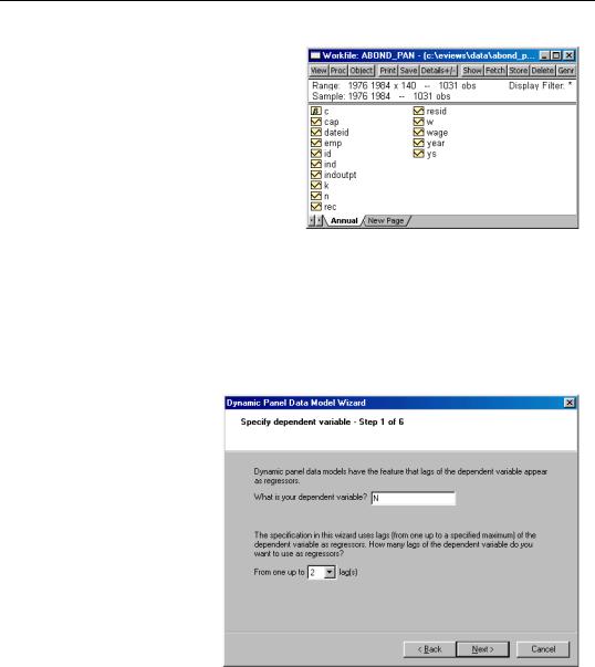
GMM Example

To illustrate the estimation of dynamic panel data models using GMM, we employ the unbalanced 1031 observation panel of firm level data from Layard and Nickell (1986), previously examined by Arellano and Bond (1991). The analysis fits the log of employment

(N) to the low of the real wage (W), log of the capital stock (K), and the log of industry output (YS).

918—Chapter 29. Panel Estimation

The workfile is structured as a dated annual panel using ID as the cross-sec- tion identifier series and YEAR as the date classification series.

Since the model is assumed to be dynamic, we employ EViews tools for estimating dynamic panel data models. To bring up the GMM dialog, enter “GMM” in the command line, or select

Quick/Estimate Equation... from the main menu, and choose GMM/DPD -

Generalized Method of Moments /Dynamic Panel Data in the Method combo box to display the IV estimator dialog.

Click on the button labeled Dynamic Panel Wizard... to bring up the DPD wizard. The DPD wizard is a tool that will aid you in filling out the general GMM dialog. The first page is an introductory screen describing the basic purpose of the wizard. Click Next to continue.

The second page of the wizard prompts you for the dependent variable and the number of its lags to include as explanatory variables. In this example, we wish to estimate an equation with N as the dependent variable and N(-1) and N(-2) as explanatory variables so we enter “N” and select “2” lags in the combo box. Click on Next to continue to the next page, where you will specify the

remaining explanatory variables.

In the third page, you will complete the specification of your explanatory variables. First, enter the list:

Panel Estimation Examples—919

w w(-1) k ys ys(-1)

in the regressor edit box to include these variables. Since the desired specification will include time dummies, make certain that the checkbox for Include period dummy variables is selected, then click on Next to proceed.

The next page of the wizard is used to specify a transformation to remove the cross-section fixed effect. You may choose to use first Differences or Orthogonal deviations. In addition, if your specification includes period dummy variables, there is a checkbox asking whether you wish to transform the period dummies, or to enter them in levels. Here we specify the first difference transforma-

tion, and choose to include untransformed period dummies in the transformed equation. Click on Next to continue.

The next page is where you will specify your dynamic period-specific (predetermined) instruments. The instruments should be entered with the “@DYN” tag to indicate that they are to be expanded into sets of predetermined instruments, with optional arguments to indicate the lags to be included. If no arguments are provided, the default is to include all valid lags (from -2 to “-infinity”).

Here, we instruct EViews that we wish to use the default lags for N as predetermined instruments.

920—Chapter 29. Panel Estimation

You should now specify the remaining instruments. There are two lists that should be provided. The first list, which is entered in the edit field labeled Transform, should contain a list of the strictly exogenous instruments that you wish to transform prior to use in estimating the transformed equation. The second list, which should be entered in the No transform edit box should contain a list of instruments that should be used directly without transformation. Enter the remaining instruments:

w w(-1) k ys ys(-1)

in the first edit box and click on Next to proceed to the final page.

The final page allows you to specify your GMM weighting and coefficient covariance calculation choices. In the first combo box, you will choose a GMM Iteration option. You may select 1-step (for i.i.d. innovations) to compute the ArellanoBond 1-step estimator, 2- step (update weights once), to compute the Arellano-Bond 2-step estimator, or n-step (iterate

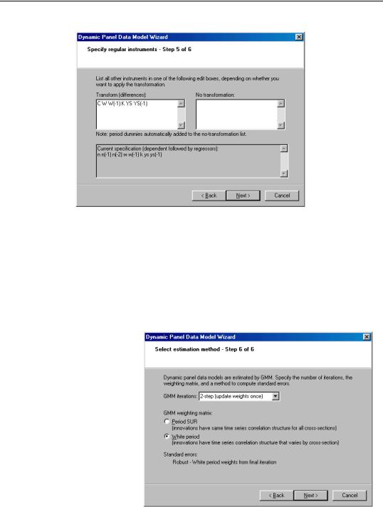
Panel Estimation Examples—921

to convergence), to iterate the weight calculations. In the first case, EViews will provide you with choices for computing the standard errors, but here only White period robust standard errors are allowed. Clicking on Next takes you to the final page. Click on Finish to return to the Equation Estimation dialog.

EViews has filled out the Equation Estimation dialog with our choices from the DPD wizard. You should take a moment to examine the settings that have been filled out for you since, in the future, you may wish to enter the specification directly into the dialog without using the wizard. You may also, of course, modify the settings in the dialog prior to continuing. For example, click on the Panel Options tab and check the No d.f. correction setting in the covariance calculation to match the original Arellano-Bond results (Table 4(b), p. 290). Click on OK to estimate the specification.

The top portion of the output describes the estimation settings, coefficient estimates, and summary statistics. Note that both the weighting matrix and covariance calculation method used are described in the top portion of the output.

Dependent Variable: N

Method: Panel Generalized Method of Moments

Transformation: First Differences

Date: 05/29/03 Time: 11:50

Sample (adjusted): 1978 1984

Number of cross-sections used: 140

Total panel (unbalanced) observations: 611

White period instrument weighting matrix

Linear estimation after one-step weighting

Instrument list: W W(-1) K YS YS(-1) @DYN(N) @LEV(@SYSPER)

Variable

Coefficient

Std. Error

t-Statistic

Prob.


N(-1)

0.474150

0.085303

5.558409

0.0000

N(-2)

-0.052968

0.027284

-1.941324

0.0527

W

-0.513205

0.049345

-10.40027

0.0000

W(-1)

0.224640

0.080063

2.805796

0.0052

K

0.292723

0.039463

7.417748

0.0000

YS

0.609775

0.108524

5.618813

0.0000

YS(-1)

-0.446371

0.124815

-3.576272

0.0004

@LEV(@ISPERIOD("1979"))

0.010509

0.007251

1.449224

0.1478

@LEV(@ISPERIOD("1980"))

0.014142

0.009959

1.420077

0.1561

@LEV(@ISPERIOD("1981"))

-0.040453

0.011551

-3.502122

0.0005

@LEV(@ISPERIOD("1982"))

-0.021640

0.011891

-1.819843

0.0693

@LEV(@ISPERIOD("1983"))

-0.001847

0.010412

-0.177358

0.8593

@LEV(@ISPERIOD("1984"))

-0.010221

0.011468

-0.891270

0.3731


Соседние файлы в папке Docs