Chapter 23. System Estimation

This chapter describes methods of estimating the parameters of systems of equations. We describe least squares, weighted least squares, seemingly unrelated regression (SUR), weighted two-stage least squares, three-stage least squares, full-information maximum likelihood (FIML), and generalized method of moments (GMM) estimation techniques.

Once you have estimated the parameters of your system of equations, you may wish to forecast future values or perform simulations for different values of the explanatory variables. Chapter 26, “Models”, on page 777 describes the use of models to forecast from an estimated system of equations or to perform single and multivariate simulation.

Background

A system is a group of equations containing unknown parameters. Systems can be estimated using a number of multivariate techniques that take into account the interdependencies among the equations in the system.

t is a vector of possibly serially correlated disturbances. The task of estimation is to find estimates of the vector of parameters β .

EViews provides you with a number of methods of estimating the parameters of the system. One approach is to estimate each equation in the system separately, using one of the single equation methods described earlier in this manual. A second approach is to estimate, simultaneously, the complete set of parameters of the equations in the system. The simultaneous approach allows you to place constraints on coefficients across equations and to employ techniques that account for correlation in the residuals across equations.

While there are important advantages to using a system to estimate your parameters, they do not come without cost. Most importantly, if you misspecify one of the equations in the system and estimate your parameters using single equation methods, only the misspecified equation will be poorly estimated. If you employ system estimation techniques, the poor estimates for the misspecification equation may “contaminate” estimates for other equations.

At this point, we take care to distinguish between systems of equations and models. A model is a group of known equations describing endogenous variables. Models are used to solve for values of the endogenous variables, given information on other variables in the model.

System Estimation Methods—697

Seemingly Unrelated Regression

The seemingly unrelated regression (SUR) method, also known as the multivariate regression, or Zellner's method, estimates the parameters of the system, accounting for heteroskedasticity and contemporaneous correlation in the errors across equations. The estimates of the cross-equation covariance matrix are based upon parameter estimates of the unweighted system.

Note that EViews estimates a more general form of SUR than is typically described in the literature, since it allows for cross-equation restrictions on parameters.

Two-Stage Least Squares

The system two-stage least squares (STSLS) estimator is the system version of the single equation two-stage least squares estimator described above. STSLS is an appropriate technique when some of the right-hand side variables are correlated with the error terms, and there is neither heteroskedasticity, nor contemporaneous correlation in the residuals. EViews estimates STSLS by applying TSLS equation by equation to the unweighted system, enforcing any cross-equation parameter restrictions. If there are no cross-equation restrictions, the results will be identical to unweighted single-equation TSLS.

Weighted Two-Stage Least Squares

The weighted two-stage least squares (WTSLS) estimator is the two-stage version of the weighted least squares estimator. WTSLS is an appropriate technique when some of the right-hand side variables are correlated with the error terms, and there is heteroskedasticity, but no contemporaneous correlation in the residuals.

EViews first applies STSLS to the unweighted system. The results from this estimation are used to form the equation weights, based upon the estimated equation variances. If there are no cross-equation restrictions, these first-stage results will be identical to unweighted single-equation TSLS.

Three-Stage Least Squares

Three-stage least squares (3SLS) is the two-stage least squares version of the SUR method. It is an appropriate technique when right-hand side variables are correlated with the error terms, and there is both heteroskedasticity, and contemporaneous correlation in the residuals.

EViews applies TSLS to the unweighted system, enforcing any cross-equation parameter restrictions. These estimates are used to form an estimate of the full cross-equation covariance matrix which, in turn, is used to transform the equations to eliminate the cross-equa- tion correlation. TSLS is applied to the transformed model.

How to Create and Specify a System—699

Consider the specification of a simple two equation system. You can use the default EViews coefficients, C(1), C(2), and so on, or you can use other coefficient vectors, in which case you should first declare them by clicking Object/

New Object.../Matrix-Vector-Coef/Coef- ficient Vector in the main menu.

There are some general rules for specifying your equations:

•Equations can be nonlinear in their variables, coefficients, or both. Cross equation coefficient restrictions may be imposed by using the same coefficients in different equations. For example:

y = c(1) + c(2)*x

z= c(3) + c(2)*z + (1-c(2))*x

•You may also impose adding up constraints. Suppose for the equation:

y= c(1)*x1 + c(2)*x2 + c(3)*x3

you wish to impose C(1)+C(2)+C(3)=1. You can impose this restriction by specifying the equation as

y= c(1)*x1 + c(2)*x2 + (1-c(1)-c(2))*x3

•The equations in a system may contain autoregressive (AR) error specifications, but not MA, SAR, or SMA error specifications. You must associate coefficients with each AR specification. Enclose the entire AR specification in square brackets and follow each AR with an “=”-sign and a coefficient. For example:

cs = c(1) + c(2)*gdp + [ar(1)=c(3), ar(2)=c(4)]

You can constrain all of the equations in a system to have the same AR coefficient by giving all equations the same AR coefficient number, or you can estimate separate AR processes, by assigning each equation its own coefficient.

•Equations in a system need not have a dependent variable followed by an equal sign and then an expression. The “=”-sign can be anywhere in the formula, as in:

log(unemp/(1-unemp)) = c(1) + c(2)*dmr

You can also write the equation as a simple expression without a dependent variable, as in:

(c(1)*x + c(2)*y + 4)^2

How to Create and Specify a System—701

Lastly, you can mix the two methods. Any equation without individually specified instruments will use the instruments specified by the @inst statement. The system:

@inst gdp(-1 to -4) x gov

cs = c(1)+c(2)*gdp+c(3)*cs(-1)

inv = c(4)+c(5)*gdp+c(6)*gov @ gdp(-1) gov

will use the instruments GDP(-1), GDP(-2), GDP(-3), GDP(-4), X, GOV, and C, for the CS equation, but only GDP(-1), GOV, and C, for the INV equation.

As noted above, the EViews default behavior is to perform the instrumental variables projection on an equation-by-equation basis. You may, however, wish to perform the projections on the stacked system. Notably, where the number of instruments is large, relative to the number of observations, stacking the equations and instruments prior to performing the projection may be the only feasible way to compute 2SLS estimates.

To designate instruments for a stacked projection, you should use the @stackinst statement (note: this statement is only available for systems estimated by 2SLS or 3SLS; it is not available for systems estimated using GMM).

In a @stackinst statement, the “@STACKINST” keyword should be followed by a list of stacked instrument specifications. Each specification is a comma delimited list of series enclosed in parentheses (one per equation), describing the instruments to be constrained in a stacked specification.

For example, the following @stackinst specification creates two instruments in a three equation model:

@stackinst (z1,z2,z3) (m1,m1,m1)

This statement instructs EViews to form two stacked instruments, one by stacking the separate series Z1, Z2, and Z3, and the other formed by stacking M1 three times. The firststage instrumental variables projection is then of the variables in the stacked system on the stacked instruments.

When working with systems that have a large number of equations, the above syntax may be unwieldy. For these cases, EViews provides a couple of shortcuts. First, for instruments that are identical in all equations, you may us an “*” after the comma to instruct EViews to repeat the specified series. Thus, the above statement is equivalent to:

@stackinst (z1,z2,z3) (m1,*)

Second, for non-identical instruments, you may specify a set of stacked instruments using an EViews group object, so long as the number of variables in the group is equal to the number of equations in the system. Thus, if you create a group Z with,

How to Create and Specify a System—703

•Identification requires that there should be at least as many instruments (including the constant) in each equation as there are right-hand side variables in that equation.

•The @stackinst statement is only available for estimation by 2SLS and 3SLS. It is not currently supported for GMM.

•If you estimate your system using a method that does not use instruments, all instrument specification lines will be ignored.

Starting Values

For systems that contain nonlinear equations, you can include a line that begins with param to provide starting values for some or all of the parameters. List pairs of parameters and values. For example:

param c(1) .15 b(3) .5

sets the initial values of C(1) and B(3). If you do not provide starting values, EViews uses the values in the current coefficient vector.

How to Estimate a System

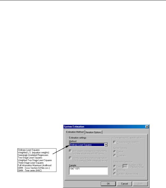
Once you have created and specified your system, you may push the Estimate button on the toolbar to bring up the System Estimation dialog.

The combo box marked Method provides you with several options for the estimation method. You may choose from one of a number of methods for estimating the parameters of your specification.

The estimation dialog may change to reflect your choice, providing you with additional options. If you select an estimator which uses instrumental variables, a checkbox will

How to Create and Specify a System—705

The Prewhitening option runs a preliminary VAR(1) prior to estimation to “soak up” the correlation in the moment conditions.

Iteration Options

For weighted least squares, SUR, weighted TSLS, 3SLS, GMM, and nonlinear systems of equations, there are additional issues involving the procedure for computing the GLS weighting matrix and the coefficient vector. To specify the method used in iteration, click on the Iteration Options tab.

The estimation option controls the method of iterating over coefficients, over the weighting matrices, or both:

•Update weights once then—Iterate coefs to convergence is the default method.

By default, EViews carries out a first-stage estimation of the coefficients using no weighting matrix (the identity matrix). Using starting

values obtained from OLS (or TSLS, if there are instruments), EViews iterates the first-stage estimates until the coefficients converge. If the specification is linear, this procedure involves a single OLS or TSLS regression.

The residuals from this first-stage iteration are used to form a consistent estimate of the weighting matrix.

In the second stage of the procedure, EViews uses the estimated weighting matrix in forming new estimates of the coefficients. If the model is nonlinear, EViews iterates the coefficient estimates until convergence.

•Update weights once then—Update coefs once performs the first-stage estimation of the coefficients, and constructs an estimate of the weighting matrix. In the second stage, EViews does not iterate the coefficients to convergence, instead performing a single coefficient iteration step. Since the first stage coefficients are consistent, this one-step update is asymptotically efficient, but unless the specification is linear, does not produce results that are identical to the first method.

•Iterate Weights and Coefs—Simultaneous updating updates both the coefficients and the weighting matrix at each iteration. These steps are then repeated until both