- •Table of Contents
- •What’s New in EViews 5.0
- •What’s New in 5.0
- •Compatibility Notes
- •EViews 5.1 Update Overview
- •Overview of EViews 5.1 New Features
- •Preface
- •Part I. EViews Fundamentals
- •Chapter 1. Introduction
- •What is EViews?
- •Installing and Running EViews
- •Windows Basics
- •The EViews Window
- •Closing EViews
- •Where to Go For Help
- •Chapter 2. A Demonstration
- •Getting Data into EViews
- •Examining the Data
- •Estimating a Regression Model
- •Specification and Hypothesis Tests
- •Modifying the Equation
- •Forecasting from an Estimated Equation
- •Additional Testing
- •Chapter 3. Workfile Basics
- •What is a Workfile?
- •Creating a Workfile
- •The Workfile Window
- •Saving a Workfile
- •Loading a Workfile
- •Multi-page Workfiles
- •Addendum: File Dialog Features
- •Chapter 4. Object Basics
- •What is an Object?
- •Basic Object Operations
- •The Object Window
- •Working with Objects
- •Chapter 5. Basic Data Handling
- •Data Objects
- •Samples
- •Sample Objects
- •Importing Data
- •Exporting Data
- •Frequency Conversion
- •Importing ASCII Text Files
- •Chapter 6. Working with Data
- •Numeric Expressions
- •Series
- •Auto-series
- •Groups
- •Scalars
- •Chapter 7. Working with Data (Advanced)
- •Auto-Updating Series
- •Alpha Series
- •Date Series
- •Value Maps
- •Chapter 8. Series Links
- •Basic Link Concepts
- •Creating a Link
- •Working with Links
- •Chapter 9. Advanced Workfiles
- •Structuring a Workfile
- •Resizing a Workfile
- •Appending to a Workfile
- •Contracting a Workfile
- •Copying from a Workfile
- •Reshaping a Workfile
- •Sorting a Workfile
- •Exporting from a Workfile
- •Chapter 10. EViews Databases
- •Database Overview
- •Database Basics
- •Working with Objects in Databases
- •Database Auto-Series
- •The Database Registry
- •Querying the Database
- •Object Aliases and Illegal Names
- •Maintaining the Database
- •Foreign Format Databases
- •Working with DRIPro Links
- •Part II. Basic Data Analysis
- •Chapter 11. Series
- •Series Views Overview
- •Spreadsheet and Graph Views
- •Descriptive Statistics
- •Tests for Descriptive Stats
- •Distribution Graphs
- •One-Way Tabulation
- •Correlogram
- •Unit Root Test
- •BDS Test
- •Properties
- •Label
- •Series Procs Overview
- •Generate by Equation
- •Resample
- •Seasonal Adjustment
- •Exponential Smoothing
- •Hodrick-Prescott Filter
- •Frequency (Band-Pass) Filter
- •Chapter 12. Groups
- •Group Views Overview
- •Group Members
- •Spreadsheet
- •Dated Data Table
- •Graphs
- •Multiple Graphs
- •Descriptive Statistics
- •Tests of Equality
- •N-Way Tabulation
- •Principal Components
- •Correlations, Covariances, and Correlograms
- •Cross Correlations and Correlograms
- •Cointegration Test
- •Unit Root Test
- •Granger Causality
- •Label
- •Group Procedures Overview
- •Chapter 13. Statistical Graphs from Series and Groups
- •Distribution Graphs of Series
- •Scatter Diagrams with Fit Lines
- •Boxplots
- •Chapter 14. Graphs, Tables, and Text Objects
- •Creating Graphs
- •Modifying Graphs
- •Multiple Graphs
- •Printing Graphs
- •Copying Graphs to the Clipboard
- •Saving Graphs to a File
- •Graph Commands
- •Creating Tables
- •Table Basics
- •Basic Table Customization
- •Customizing Table Cells
- •Copying Tables to the Clipboard
- •Saving Tables to a File
- •Table Commands
- •Text Objects
- •Part III. Basic Single Equation Analysis
- •Chapter 15. Basic Regression
- •Equation Objects
- •Specifying an Equation in EViews
- •Estimating an Equation in EViews
- •Equation Output
- •Working with Equations
- •Estimation Problems
- •Chapter 16. Additional Regression Methods
- •Special Equation Terms
- •Weighted Least Squares
- •Heteroskedasticity and Autocorrelation Consistent Covariances
- •Two-stage Least Squares
- •Nonlinear Least Squares
- •Generalized Method of Moments (GMM)
- •Chapter 17. Time Series Regression
- •Serial Correlation Theory
- •Testing for Serial Correlation
- •Estimating AR Models
- •ARIMA Theory
- •Estimating ARIMA Models
- •ARMA Equation Diagnostics
- •Nonstationary Time Series
- •Unit Root Tests
- •Panel Unit Root Tests
- •Chapter 18. Forecasting from an Equation
- •Forecasting from Equations in EViews
- •An Illustration
- •Forecast Basics
- •Forecasting with ARMA Errors
- •Forecasting from Equations with Expressions
- •Forecasting with Expression and PDL Specifications
- •Chapter 19. Specification and Diagnostic Tests
- •Background
- •Coefficient Tests
- •Residual Tests
- •Specification and Stability Tests
- •Applications
- •Part IV. Advanced Single Equation Analysis
- •Chapter 20. ARCH and GARCH Estimation
- •Basic ARCH Specifications
- •Estimating ARCH Models in EViews
- •Working with ARCH Models
- •Additional ARCH Models
- •Examples
- •Binary Dependent Variable Models
- •Estimating Binary Models in EViews
- •Procedures for Binary Equations
- •Ordered Dependent Variable Models
- •Estimating Ordered Models in EViews
- •Views of Ordered Equations
- •Procedures for Ordered Equations
- •Censored Regression Models
- •Estimating Censored Models in EViews
- •Procedures for Censored Equations
- •Truncated Regression Models
- •Procedures for Truncated Equations
- •Count Models
- •Views of Count Models
- •Procedures for Count Models
- •Demonstrations
- •Technical Notes
- •Chapter 22. The Log Likelihood (LogL) Object
- •Overview
- •Specification
- •Estimation
- •LogL Views
- •LogL Procs
- •Troubleshooting
- •Limitations
- •Examples
- •Part V. Multiple Equation Analysis
- •Chapter 23. System Estimation
- •Background
- •System Estimation Methods
- •How to Create and Specify a System
- •Working With Systems
- •Technical Discussion
- •Vector Autoregressions (VARs)
- •Estimating a VAR in EViews
- •VAR Estimation Output
- •Views and Procs of a VAR
- •Structural (Identified) VARs
- •Cointegration Test
- •Vector Error Correction (VEC) Models
- •A Note on Version Compatibility
- •Chapter 25. State Space Models and the Kalman Filter
- •Background
- •Specifying a State Space Model in EViews
- •Working with the State Space
- •Converting from Version 3 Sspace
- •Technical Discussion
- •Chapter 26. Models
- •Overview
- •An Example Model
- •Building a Model
- •Working with the Model Structure
- •Specifying Scenarios
- •Using Add Factors
- •Solving the Model
- •Working with the Model Data
- •Part VI. Panel and Pooled Data
- •Chapter 27. Pooled Time Series, Cross-Section Data
- •The Pool Workfile
- •The Pool Object
- •Pooled Data
- •Setting up a Pool Workfile
- •Working with Pooled Data
- •Pooled Estimation
- •Chapter 28. Working with Panel Data
- •Structuring a Panel Workfile
- •Panel Workfile Display
- •Panel Workfile Information
- •Working with Panel Data
- •Basic Panel Analysis
- •Chapter 29. Panel Estimation
- •Estimating a Panel Equation
- •Panel Estimation Examples
- •Panel Equation Testing
- •Estimation Background
- •Appendix A. Global Options
- •The Options Menu
- •Print Setup
- •Appendix B. Wildcards
- •Wildcard Expressions
- •Using Wildcard Expressions
- •Source and Destination Patterns
- •Resolving Ambiguities
- •Wildcard versus Pool Identifier
- •Appendix C. Estimation and Solution Options
- •Setting Estimation Options
- •Optimization Algorithms
- •Nonlinear Equation Solution Methods
- •Appendix D. Gradients and Derivatives
- •Gradients
- •Derivatives
- •Appendix E. Information Criteria
- •Definitions
- •Using Information Criteria as a Guide to Model Selection
- •References
- •Index
- •Symbols
- •.DB? files 266
- •.EDB file 262
- •.RTF file 437
- •.WF1 file 62
- •@obsnum
- •Panel
- •@unmaptxt 174
- •~, in backup file name 62, 939
- •Numerics
- •3sls (three-stage least squares) 697, 716
- •Abort key 21
- •ARIMA models 501
- •ASCII
- •file export 115
- •ASCII file
- •See also Unit root tests.
- •Auto-search
- •Auto-series
- •in groups 144
- •Auto-updating series
- •and databases 152
- •Backcast
- •Berndt-Hall-Hall-Hausman (BHHH). See Optimization algorithms.
- •Bias proportion 554
- •fitted index 634
- •Binning option
- •classifications 313, 382
- •Boxplots 409
- •By-group statistics 312, 886, 893
- •coef vector 444
- •Causality
- •Granger's test 389
- •scale factor 649
- •Census X11
- •Census X12 337
- •Chi-square
- •Cholesky factor
- •Classification table
- •Close
- •Coef (coefficient vector)
- •default 444
- •Coefficient
- •Comparison operators
- •Conditional standard deviation
- •graph 610
- •Confidence interval
- •Constant
- •Copy
- •data cut-and-paste 107
- •table to clipboard 437
- •Covariance matrix
- •HAC (Newey-West) 473
- •heteroskedasticity consistent of estimated coefficients 472
- •Create
- •Cross-equation
- •Tukey option 393
- •CUSUM
- •sum of recursive residuals test 589
- •sum of recursive squared residuals test 590
- •Data
- •Database
- •link options 303
- •using auto-updating series with 152
- •Dates
- •Default
- •database 24, 266
- •set directory 71
- •Dependent variable
- •Description
- •Descriptive statistics
- •by group 312
- •group 379
- •individual samples (group) 379
- •Display format
- •Display name
- •Distribution
- •Dummy variables
- •for regression 452
- •lagged dependent variable 495
- •Dynamic forecasting 556
- •Edit
- •See also Unit root tests.
- •Equation
- •create 443
- •store 458
- •Estimation
- •EViews
- •Excel file
- •Excel files
- •Expectation-prediction table
- •Expected dependent variable
- •double 352
- •Export data 114
- •Extreme value
- •binary model 624
- •Fetch
- •File
- •save table to 438
- •Files
- •Fitted index
- •Fitted values
- •Font options
- •Fonts
- •Forecast
- •evaluation 553
- •Foreign data
- •Formula
- •forecast 561
- •Freq
- •DRI database 303
- •F-test
- •for variance equality 321
- •Full information maximum likelihood 698
- •GARCH 601
- •ARCH-M model 603
- •variance factor 668
- •system 716
- •Goodness-of-fit
- •Gradients 963
- •Graph
- •remove elements 423
- •Groups
- •display format 94
- •Groupwise heteroskedasticity 380
- •Help
- •Heteroskedasticity and autocorrelation consistent covariance (HAC) 473
- •History
- •Holt-Winters
- •Hypothesis tests
- •F-test 321
- •Identification
- •Identity
- •Import
- •Import data
- •See also VAR.
- •Index
- •Insert
- •Instruments 474
- •Iteration
- •Iteration option 953
- •in nonlinear least squares 483
- •J-statistic 491
- •J-test 596
- •Kernel
- •bivariate fit 405
- •choice in HAC weighting 704, 718
- •Kernel function
- •Keyboard
- •Kwiatkowski, Phillips, Schmidt, and Shin test 525
- •Label 82
- •Last_update
- •Last_write
- •Latent variable
- •Lead
- •make covariance matrix 643
- •List
- •LM test
- •ARCH 582
- •for binary models 622
- •LOWESS. See also LOESS
- •in ARIMA models 501
- •Mean absolute error 553
- •Metafile
- •Micro TSP
- •recoding 137
- •Models
- •add factors 777, 802
- •solving 804
- •Mouse 18
- •Multicollinearity 460
- •Name
- •Newey-West
- •Nonlinear coefficient restriction
- •Wald test 575
- •weighted two stage 486
- •Normal distribution
- •Numbers
- •chi-square tests 383
- •Object 73
- •Open
- •Option setting
- •Option settings
- •Or operator 98, 133
- •Ordinary residual
- •Panel
- •irregular 214
- •unit root tests 530
- •Paste 83
- •PcGive data 293
- •Polynomial distributed lag
- •Pool
- •Pool (object)
- •PostScript
- •Prediction table
- •Principal components 385
- •Program
- •p-value 569
- •for coefficient t-statistic 450
- •Quiet mode 939
- •RATS data
- •Read 832
- •CUSUM 589
- •Regression
- •Relational operators
- •Remarks
- •database 287
- •Residuals
- •Resize
- •Results
- •RichText Format
- •Robust standard errors
- •Robustness iterations
- •for regression 451
- •with AR specification 500
- •workfile 95
- •Save
- •Seasonal
- •Seasonal graphs 310
- •Select
- •single item 20
- •Serial correlation
- •theory 493
- •Series
- •Smoothing
- •Solve
- •Source
- •Specification test
- •Spreadsheet
- •Standard error
- •Standard error
- •binary models 634
- •Start
- •Starting values
- •Summary statistics
- •for regression variables 451
- •System
- •Table 429
- •font 434
- •Tabulation
- •Template 424
- •Tests. See also Hypothesis tests, Specification test and Goodness of fit.
- •Text file
- •open as workfile 54
- •Type
- •field in database query 282
- •Units
- •Update
- •Valmap
- •find label for value 173
- •find numeric value for label 174
- •Value maps 163
- •estimating 749
- •View
- •Wald test 572
- •nonlinear restriction 575
- •Watson test 323
- •Weighting matrix
- •heteroskedasticity and autocorrelation consistent (HAC) 718
- •kernel options 718
- •White
- •Window
- •Workfile
- •storage defaults 940
- •Write 844
- •XY line
- •Yates' continuity correction 321
Chapter 2. A Demonstration
In this chapter, we provide a demonstration of some basic features of EViews. The demonstration is meant to be a brief introduction to EViews; not a comprehensive description of the program. A full description of the program begins in Chapter 4, “Object Basics”, on page 73.
This demo takes you through the following steps:
•getting data into EViews from an Excel spreadsheet
•examining your data and performing simple statistical analyses
•using regression analysis to model and forecast a statistical relationship
•performing specification and hypothesis testing
•plotting results
Getting Data into EViews
The first step in most projects will be to read your data into an EViews workfile. EViews provides sophisticated tools for reading from a variety of common data formats, making it extremely easy to get started.
Before we describe the process of reading a foreign data file, note that the data for this demonstration have been included in both Excel spreadsheet and EViews workfile formats in your EViews installation directory (“./Example Files/Data”). If you wish to skip the discussion of opening foreign files, going directly to the analysis part of the demonstration, you may load the EViews workfile by selecting File/Open/Foreign Data as Workfile… and opening DEMO.WF1.
28—Chapter 2. A Demonstration
The easiest way to open the Excel file DEMO.XLS, is to drag- and-drop the file into an open EViews application window. You may also drag-and-drop the file onto the EViews icon. Windows will first start the EViews application and will then open the demonstration Excel workfile.
Alternately, you may use the
File/Open/EViews workfile...
dialog, selecting Files of type Excel and selecting the desired file.
As EViews opens the file, the program determines that the file is in Excel file format, analyzes the contents of the file, and opens the Excel Read wizard.
The first page of the wizard includes a preview of the data found in the spreadsheet. In most cases, you need not worry about any of the options on this page. In more complicated cases, you may use the options on this page to provide a custom range of cells to read, or to select a different sheet in the workbook.
The second page of the wizard contains various options for reading the Excel data. These options are set at the most likely choices given the EViews analysis of the contents of your workbook. In most cases, you should simply click on Finish to accept the default settings. In other cases where the preview window does not correctly display the desired data, you may click on Next and adjust the options that appear on the second page of the wizard. In our example, the data appear to be correct, so we simply click on Finish to accept the default settings.
Getting Data into EViews—29
When you accept the settings, EViews automatically creates a workfile that is sized to hold the data, and imports the series into the workfile. The workfile ranges from 1952 quarter 1 to 1996 quarter 4, and contains five series (GDP, M1, OBS, PR, and RS) that you have read from the Excel file. There are also two objects, the coefficient vector C and the series RESID, that are found in all EViews workfiles.
In addition, EViews opens the imported data in a spreadsheet view, allowing you to perform a initial examination of your data. You should compare the spreadsheet views with the Excel worksheet to ensure that the data have been read correctly. You can use the scroll bars and scroll arrows on the right side of the window to view and verify the reminder of the data.
You may wish to click on Name in the group toolbar to provide a name for your UNTITLED group. Enter the name ORIGINAL, and click on OK to accept the name.
Once you are satisfied that the data are correct, you should save the workfile by clicking on the Save button in the workfile window. A saved dialog will open, prompting you for a workfile name and location. You should enter DEMO2.WF1, and then click OK. A second dialog may be displayed prompting you to set storage options. Click OK to accept the defaults. EViews will save the workfile in the specified directory with the name DEMO2.WF1. A saved workfile may be opened later by selecting File/Open/Workfile.… from the main menu.
30—Chapter 2. A Demonstration
Examining the Data
Now that you have your data in an EViews workfile, you may use basic EViews tools to examine the data in your series and groups in a variety of ways.
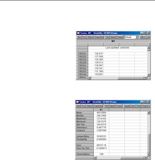
First, we examine the characteristics of individual series. To see the contents of the M1 series, simply double click on the M1 icon in the workfile window, or select Quick/Show… in the main menu, enter m1, and click
OK.
EViews will open the M1 series object and will display the default spreadsheet view of the series. Note the description of the contents of the
series (“Series: M1”) in the upper leftmost corner of the series window toolbar, indicating that you are working with the M1 series.
You will use the entries in the View and Proc menus to examine various characteristics of the series. Simply click on the buttons on the toolbar to access these menu entries, or equivalently, select View or Proc from the main menu.
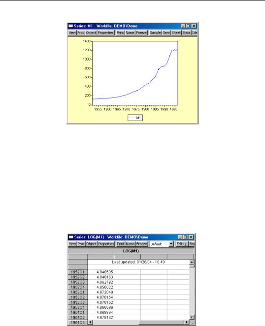
To compute, for example, a table of basic descriptive statistics for M1, simply click on the View button, then select Descriptive Statistics/ Stats Table. EViews will compute descriptive statistics for M1 and
change the series view to display a table of results.
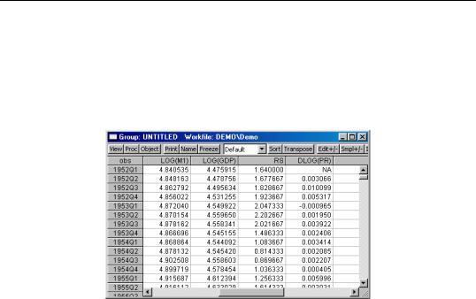
Similarly, to examine a line graph of the series, simply select View/Graph/Line. EViews will change the M1 series window to display a line graph of the data in the M1 series.
Examining the Data—31
At this point, you may wish to explore the contents of the View and Proc menus in the M1 series window to see the various tools for examining and working with series data. You may always return to the spreadsheet view of your series by selecting View/Spreadsheet from the toolbar or main menu.
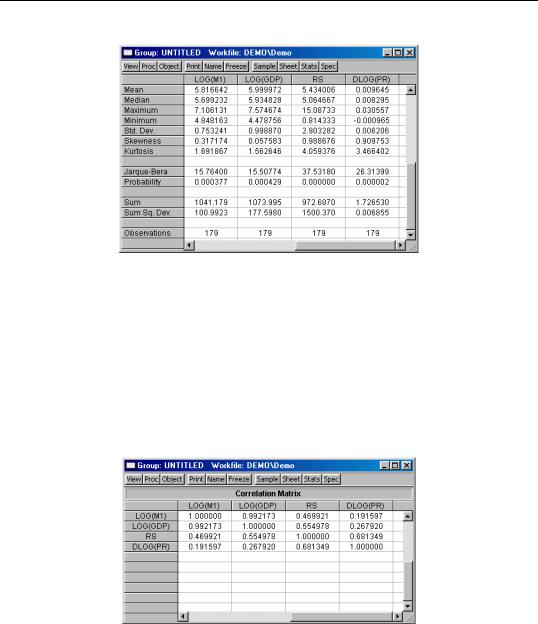
Since our ultimate goal is to perform regression analysis with our data expressed in natural logarithms, we may instead wish to work with the log of M1. Fortunately, EViews allows you to work with expressions involving series as easily as you work with the series themselves. To open a series containing this expression, select Quick/Show… from the main menu, enter the text for the expression, log(m1), and click OK. EViews will open a series window for containing LOG(M1). Note that the titlebar for the series shows that we are working with the desired expression.
You may work with this auto-series in exactly the same way you worked with M1 above. For example, clicking on View in the series toolbar and selecting Descriptive Statistics/
32—Chapter 2. A Demonstration
Histogram and Stats displays a view containing a histogram and descriptive statistics for LOG(M1):
Alternately, we may display a smoothed version of the histogram by selecting View/Distribution Graphs/Kernel Density… and clicking on OK to accept the default options:
Suppose that you wish to examine multiple series or series expressions. To do so, you will need to construct a group object that contains the series of interest.
Earlier, you worked with an EViews created group object containing all of the series read from your Excel file. Here, we will construct a group object containing expressions involving a subset of those series. We wish to create a group object containing the logarithms of the series M1 and GDP, the level of RS, and the first difference of the logarithm of the
Examining the Data—33
series PR. Simply select Quick/Show... from the main EViews menu, and enter the list of expressions and series names:
log(m1) log(gdp) rs dlog(pr)
Click on OK to accept the input. EViews will open a group window containing a spreadsheet view of the series and expressions of interest.
As with the series object, you will use the View and Proc menus of the group to examine various characteristics of the group of series. Simply click on the buttons on the toolbar to access these menu entries or select View or Proc from the main menu to call up the relevant entries. Note that the entries for a group object will differ from those for a series object since the kinds of operations you may perform with multiple series differ from the types of operations available when working with a single series.
For example, you may select View/Graphs/Line from the group object toolbar to display a single graph containing line plots of each of the series in the group:
34—Chapter 2. A Demonstration
Alternately, you may select View/Multiple Graphs/Line to display the same information, but with each series expression plotted in an individual graph:
Likewise, you may select View/Descriptive Stats/Individual Samples to display a table of descriptive statistics computed for each of the series in the group:
Examining the Data—35
Note that the number of observations used for computing descriptive statistics for DLOG(PR) is one less than the number used to compute the statistics for the other expressions. By electing to compute our statistics using “Individual Samples”, we informed EViews that we wished to use the series specific samples in each computation, so that the loss of an observation in DLOG(PR) to differencing should not affect the samples used in calculations for the remaining expressions.
We may instead choose to use “Common Samples” so that observations are only used if the data are available for all of the series in the group. Click on View/Correlations/Common Samples to display the correlation matrix of the four series for the 179 common observations:
Once again, we suggest that you may wish to explore the contents of the View and Proc menus for this group to see the various tools for examining and working with sets of series You can always return to the spreadsheet view of the group by selecting View/Spreadsheet.