Tests for Descriptive Stats

316—Chapter 11. Series

where X is the sample mean of X, s is the unbiased sample standard deviation, and N is the number of observations of X. If X is normally distributed, under the null hypothesis the t-statistic follows a t-distribution with N − 1 degrees of freedom.

If you specify a value for the standard deviation of X, EViews also reports a z-statistic:

where σ is the specified standard deviation of X. If X is normally distributed with standard deviation σ , under the null hypothesis, the z-statistic has a standard normal distribution.

To carry out the mean test, type in the value of the mean under the null hypothesis in the edit field next to Mean. If you want to compute the z-statistic conditional on a known standard deviation, also type in a value for the standard deviation in the right edit field. You can type in any number or standard EViews expression in the edit fields.

The reported probability value is the p-value, or marginal significance level, against a twosided alternative. If this probability value is less than the size of the test, say 0.05, we reject the null hypothesis. Here, we strongly reject the null hypothesis for the two-sided test of equality. The probability value for a one-sided alternative is one half the p-value of the two-sided test.

Variance Test

Carries out the test of the null hypothesis that the variance of a series X is equal to a specified value σ2 against the two-sided alternative that it is not equal to σ2 :

H0: var( x) = σ2

(11.8)

H1: var( x) ≠ σ2.

where N is the number of observations, s is the sample standard deviation, and X is the sample mean of X. Under the null hypothesis and the assumption that X is normally distributed, the statistic follows a χ2 distribution with N − 1 degrees of freedom. The probability value is computed as min ( p, 1 − p) , where p is the probability of observing a χ2 - statistic as large as the one actually observed under the null hypothesis.

To carry out the variance test, type in the value of the variance under the null hypothesis in the field box next to Variance. You can type in any positive number or expression in the field.

Median Test

EViews reports three rank-based, nonparametric test statistics. The principal references for this material are Conover (1980) and Sheskin (1997).

•Binomial sign test. This test is based on the idea that if the sample is drawn randomly from a binomial distribution, the sample proportion above and below the true median should be one-half. Note that EViews reports two-sided p-values for both the sign test and the large sample normal approximation (with continuity correction).

•Wilcoxon signed ranks test. Suppose that we compute the absolute value of the difference between each observation and the mean, and then rank these observations from high to low. The Wilcoxon test is based on the idea that the sum of the ranks for the samples above and below the median should be similar. EViews reports a p- value for the asymptotic normal approximation to the Wilcoxon T-statistic (correcting for both continuity and ties). See Sheskin (1997, pp. 82–94) and Conover (1980, p. 284).

•Van der Waerden (normal scores) test. This test is based on the same general idea as the Wilcoxon test, but is based on smoothed ranks. The signed ranks are smoothed by converting them to quantiles of the normal distribution (normal scores). EViews reports the two-sided p-value for the asymptotic normal test described by Conover (1980).

318—Chapter 11. Series

To carry out the median test, type in the value of the median under the null hypothesis in the edit box next to Median. You can type any numeric expression in the edit field.

Hypothesis Testing for LWAGE

Date: 10/14/97 Time: 23:23

Sample: 1 1000

Included observations: 1000

Test of Hypothesis: Median = 2.25

Sample Median = 2.302585

Median Test Summary

Equality Tests by Classification

This view allows you to test equality of the means, medians, and variances across subsamples (or subgroups) of a single series. For example, you can test whether mean income is the same for males and females, or whether the variance of education is related to race. The tests assume that the subsamples are independent.

For single sample tests, see the discussion of “Simple Hypothesis Tests” on page 315. For tests of equality across different series, see “Tests of Equality” on page 380.

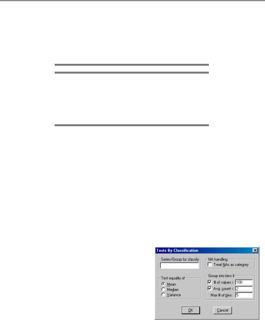
Select View/Tests for Descriptive Stats/Equality Tests by Classification… and the Tests by Classification dialog box appears.

First, select whether you wish to test the mean, the median or the variance. Specify the subgroups, the NA handling, and the grouping options as described in “Stats by Classification” beginning on page 312.

Mean Equality Test

This test is based on a single-factor, between-subjects, analysis of variance (ANOVA). The basic idea is that if the subgroups have the same mean, then the variability between the

320—Chapter 11. Series

The analysis of variance table shows the decomposition of the total sum of squares into the between and within sum of squares, where:

Mean Sq. = Sum of Sq./df

The F-statistic is the ratio:

F = Between Mean Sq./Within Mean Sq.

The bottom portion of the output provides the category statistics:

Category Statistics

Median (Distribution) Equality Tests

EViews computes various rank-based nonparametric tests of the hypothesis that the subgroups have the same general distribution, against the alternative that at least one subgroup has a different distribution.

In the two group setting, the null hypothesis is that the two subgroups are independent samples from the same general distribution. The alternative hypothesis may loosely be defined as “the values [of the first group] tend to differ from the values [of the second group]” (see Conover 1980, p. 281 for discussion). See also Bergmann, Ludbrook and Spooren (2000) for a more precise analysis of the issues involved.

We note that the “median” category in which we place these tests is somewhat misleading since the tests focus more generally on the equality of various statistics computed across subgroups. For example, the Wilcoxon test examines the comparability of mean ranks across subgroups. The categorization reflects common usage for these tests and various textbook definitions. The tests may, of course, have power against median differences.

•Wilcoxon signed ranks test. This test is computed when there are two subgroups. The test is identical to the Wilcoxon test outlined in the description of median tests (“Median Test” on page 317) but the division of the series into two groups is based upon the values of the classification variable instead of the value of the observation relative to the median.