356—Chapter 11. Series

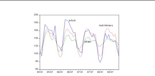
The forecasts from the multiplicative exponential smoothing method do a good job of tracking the seasonal movements in the actual series.

Hodrick-Prescott Filter

The Hodrick-Prescott Filter is a smoothing method that is widely used among macroeconomists to obtain a smooth estimate of the long-term trend component of a series. The method was first used in a working paper (circulated in the early 1980’s and published in 1997) by Hodrick and Prescott to analyze postwar U.S. business cycles.

Technically, the Hodrick-Prescott (HP) filter is a two-sided linear filter that computes the smoothed series s of y by minimizing the variance of y around s , subject to a penalty that constrains the second difference of s . That is, the HP filter chooses s to minimize:

The penalty parameter λ controls the smoothness of the series σ . The larger the λ , the smoother the σ . As λ = ∞ , s approaches a linear trend.

To smooth the series using the Hodrick-Prescott filter, choose Proc/Hodrick-Prescott Filter…:

358—Chapter 11. Series

range. If you are working with quarterly data, this range corresponds to a low duration of 6, and an upper duration of 32 quarters. Thus, you should set PL = 6 and PU = 32 .

In some contexts, it will be useful to think in terms of frequencies which describe the number of cycles in a given period (obviously, periodicities and frequencies are inversely related). By convention, we will say that periodicities in the range (PL, PU) correspond to frequencies in the range (2π ⁄ PU, 2π ⁄ PL) .

Note that since saying that we have a cycle with a period of 1 is meaningless, we require that 2 ≤ PL < PU . Setting PL to the lower-bound value of 2 yields a high-pass filter in which all frequencies above 2π ⁄ PU are passed through.

The various band-pass filters differ in the way that they compute the moving average:

•The fixed length symmetric filters employ a fixed lead/lag length. Here, the user must specify the fixed number of lead and lag terms to be used when computing the weighted moving average. The symmetric filters are time-invariant since the moving average weights depend only on the specified frequency band, and do not use the data. EViews computes two variants of this filter, the first due to Baxter-King (1999) (BK), and the second to Christiano-Fitzgerald (2003) (CF). The two forms differ in the choice of objective function used to select the moving average weights.

•Full sample asymmetric – this is the most general filter, where the weights on the leads and lags are allowed to differ. The asymmetric filter is time-varying with the weights both depending on the data and changing for each observation. EViews computes the Christiano-Fitzgerald (CF) form of this filter.

In choosing between the two methods, bear in mind that the fixed length filters require that we use same number of lead and lag terms for every weighted moving average. Thus, a filtered series computed using q leads and lags observations will lose q observations from both the beginning and end of the original sample. In contrast, the asymmetric filtered series do not have this requirement and can be computed to the ends of the original sample.

Computing a Band-Pass Filter in EViews

The band-pass filter is available as a series Proc in EViews. To display the band-pass filter dialog, select Proc/Frequency Filter... from the main series menu.

The first thing you will do is to select a filter type. There are three types: Fixed length symmetric (Baxter-King), Fixed length symmetric (Christiano-Fitzgerald), or Full length asymmetric (Christiano-Fitzgerald). By default, the EViews will compute the Bax- ter-King fixed length symmetric filter.

360—Chapter 11. Series

The Filter Output

Here, we depict the output from the Baxter-King filter. The left panel depicts the original series, filtered series, and the non-cyclical component (difference between the original and the filtered).

For the BK and CF fixed length symmetric filters, EViews plots the frequency response function α( ω) representing the extent to which the filtered series “responds” to the original series at frequency ω . At a given frequency ω , α( ω) 2 indicates the extent to which a moving average raises or lowers the variance of the filtered series relative to that of the original series. The right panel of the graph depicts the function. Note that the horizontal axis of a frequency response function is always in the range 0 to 0.5, in units of cycles per duration. Thus, as depicted in the graph, the frequency response function of the ideal band-pass filter for periodicities ( PL, PU) will be one in the range ( 1 ⁄ PU, 1 ⁄ PL) .

The frequency response function is not drawn for the CF time-varying filter since these filters vary with the data and observation number. If you wish to plot the frequency response function for a particular observation, you will have to save the weight matrix and then evaluate the frequency response in a separate step. The example program BFP02.PRG and subroutine FREQRESP.PRG illustrate the steps in computing of gain functions for timevarying filters at particular observations.

The Weight Matrix

For time-invariant (fixed-length symmetric) filters, the weight matrix is of dimension

1 × ( q + 1 ) where q is the user-specified lag length order. For these filters, the weights on the leads and the lags are the same, so the returned matrix contains only the one-sided weights. The filtered series can be computed as: