


Samples—95
expressions to be included in the group. This method differs from using Object/New Object… only in that it does not allow you to name the object at the time it is created.
You can also create an empty group that may be used for entering new data from the keyboard or pasting data copied from another Windows program. These methods are described in detail in “Entering Data” on page 106 and “Copying-and-Pasting” on page 107.
Editing in a Group
Editing data in a group is similar to editing data in a series. Open the group window, and click on Sheet, if necessary, to display the spreadsheet view. If the group spreadsheet is in protected mode, click on Edit +/– to enable edit mode, then select a cell to edit, enter the new value, and press RETURN. The new number should appear in the spreadsheet.
Since groups are simply references to series, editing the series within a group changes the values in the original series.
As with series spreadsheet views, you may click on Smpl +/– to toggle between showing all of the observations in the workfile and showing only those observations in the current sample. Unlike the series window, the group window always shows series in a single column.
Note that while groups inherit many of the series display formats when they are created, to reduce confusion, groups do not initially show transformed values of the series. If you wish to edit a series in a group in transformed form, you must explicitly set a transformation type for the group display.
Samples
One of the most important concepts in EViews is the sample of observations. The sample is the set (often a subset) of observations in the workfile to be included in data display and in performing statistical procedures. Samples may be specified using ranges of observations and “if conditions” that observations must satisfy to be included.
For example, you can tell EViews that you want to work with observations from 1953M1 to 1970M12 and 1995M1 to 1996M12. Or you may want to work with data from 1953M1 to 1958M12 where observations in the RC series exceed 3.6.
The remainder of this discussion describes the basics of using samples in non-panel workfiles. For a discussion of panel samples, see “Panel Samples” beginning on page 881.
The Workfile Sample
When you create a workfile, the workfile sample or global sample is set initially to be the entire range of the workfile. The workfile sample tells EViews what set of observations you
96—Chapter 5. Basic Data Handling
wish to use for subsequent operations. Unless you want to work with a different set of observations, you will not need to reset the workfile sample.
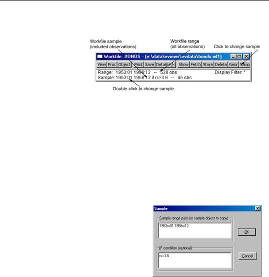
You can always determine the current workfile sample of observations by looking at the top of your workfile window.
Here the BONDS
workfile consists of 528 observations from January 1953 to December 1996. The current workfile sample uses a subset of those observations consisting of the 45 observations between 1953:01 and 1958:12 for which the value of the RC series exceeds 3.6.
Changing the Sample
There are four ways to set the workfile sample: you may click on the Sample button in the workfile toolbar, you may double click on the sample string display in the workfile window, you can select Proc/Sample… from the main workfile menu, or you may enter a smpl command in the command window. If you use one of the interactive methods, EViews will open the Sample dialog prompting you for input.
Date Pairs
In the upper edit field you will enter one or more pairs of dates (or observation numbers). Each pair identifies a starting and ending observation for a range to be included in the sample.
For example, if, in an annual workfile, you entered the string “1950 1980 1990 1995”, EViews will use observations for 1950 through 1980 and observations for 1990
through 1995 in subsequent operations; observations from 1981 through 1989 will be excluded. For undated data, the date pairs correspond to observation identifiers such as “1 50” for the first 50 observations.
You may enter your date pairs in a frequency other than that of the workfile. Dates used for the starts of date pairs are rounded down to the first instance of the corresponding date in the workfile frequency, while dates used for the ends of date pairs are rounded up to the last instance of the corresponding date in the workfile frequency. For example, the date pair “1990m1 2002q3” in an annual workfile will be rounded to “1990 2002”, while the

Samples—97
date pair “1/30/2003 7/20/2004” in a quarterly workfile will be rounded to “2003q1 2004q3”.
EViews provides special keywords that may make entering sample date pairs easier. First, you can use the keyword “@ALL”, to refer to the entire workfile range. In the workfile above, entering “@ALL” in the dialog is equivalent to entering “1953M1 1996M12”. Furthermore, you may use “@FIRST” and “@LAST” to refer to the first and last observation in the workfile. Thus, the three sample specifications for the above workfile:
@all
@first 1996m12
1953m1 @last
are identical.
Note that when interpreting sample specifications involving days, EViews will, if necessary, use the global defaults (“Dates & Frequency Conversion” on page 939) to determine the correct ordering of days, months, and years. For example, the order of the months and years is ambiguous in the date pair:
1/3/91 7/5/95
so EViews will use the default date settings to determine the desired ordering. We caution you, however, that using the default settings to disambiguate dates in samples is not generally a good idea since a given pair may be interpreted in different ways at different times if your settings change.
Alternately, you may use the IEEE standard format, “YYYY-MM-DD”, which uses a fourdigit year, followed by a dash, a two-digit month, a second dash, and a two-digit day. The presence of a dash in the format means that you must enclose the date in quotes for EViews to accept this format. For example:
"1991-01-03" "1995-07-05"
will always be interpreted as January 3, 1991 and July 5, 1995. See “Free-format Conversion Details” on page 149 of the Command and Programming Reference for related discussion.
Sample IF conditions
The lower part of the sample dialog allows you to add conditions to the sample specification. The sample is the intersection of the set of observations defined by the range pairs in the upper window and the set of observations defined by the “if” conditions in the lower window. For example, if you enter:
Upper window: 1980 1993
Lower window: incm > 5000

98—Chapter 5. Basic Data Handling
the sample includes observations for 1980 through 1993 where the series INCM is greater than 5000.
Similarly, if you enter:
Upper window: 1958q1 1998q4
Lower window: gdp > gdp(-1)
all observations from the first quarter of 1958 to the last quarter of 1998, where GDP has risen from the previous quarter, will be included.
The “or” and “and” operators allow for the construction of more complex expressions. For example, suppose you now wanted to include in your analysis only those individuals whose income exceeds 5000 dollars per year and who have at least 13 years of education. Then you can enter:
Upper window: @all
Lower window: income > 5000 and educ >= 13
Multiple range pairs and “if” conditions may also be specified:
Upper window: 50 100 200 250
Lower window: income >= 4000 and educ > 12
includes undated workfile observations 50 through 100 and 200 through 250, where the series INCOME is greater than or equal to 4000 and the series EDUC is greater than 12.
You can create even more elaborate selection rules by including EViews built-in functions: Upper window: 1958m1 1998m1
Lower window: (ed>=6 and ed<=13) or earn<@mean(earn)
includes all observations where the value of the variable ED falls between 6 and 13, or where the value of the variable EARN is lower than its mean. Note that you may use parentheses to group the conditions and operators when there is potential ambiguity in the order of evaluation.
It is possible that one of the comparisons used in the conditioning statement will generate a missing value. For example, if an observation on INCM is missing, then the comparison INCM>5000 is not defined for that observation. EViews will treat such missing values as though the condition were false, and the observation will not be included in the sample.
Sample Commands
You may find it easier to set your workfile sample from the command window—instead of using the dialog, you may set the active sample using the smpl command. Simply click on the command window to make it active, and type the keyword “SMPL”, followed by the sample string:
Samples—99
smpl 1955m1 1958m12 if rc>3.6
and then press ENTER (notice, in the example above, the use of the keyword “IF” to separate the two parts of the sample specification). You should see the sample change in the workfile window.
Sample Offsets
Sample range elements may contain mathematical expressions to create date offsets. This feature can be particularly useful in setting up a fixed width window of observations. For example, in the regular frequency monthly workfile above, the sample string:
1953m1 1953m1+11
defines a sample that includes the 12 observations in the calendar year beginning in 1953M1.
While EViews expects date offsets that are integer values, there is nothing to stop you from adding or subtracting non-integer values—EViews will automatically convert the number to an integer. You should be warned, however, that the conversion behavior is not guaranteed to be well-defined. If you must use non-integer values, you are strongly encouraged to use the “@ROUND”, “@FLOOR” or “@CEIL” functions to enforce the desired behavior.
The offsets are perhaps most useful when combined with the special keywords to trim observations from the beginning or end of the sample. For example, to drop the first observation in your sample, you may use the sample statement:
smpl @first+1 @last
Accordingly, the following commands generate a series containing cumulative sums of the series X in XSUM:
smpl @first @first
series xsum = x
smpl @first+1 @last
xsum = xsum(-1) + x
(see “Basic Assignment” on page 138). The first two commands initialize the cumulative sum for the first observation in each cross-section. The last two commands accumulate the sum of values of X over the remaining observations.
Similarly, if you wish to estimate your equation on a subsample of data and then perform cross-validation on the last 20 observations, you may use the sample defined by,
smpl @first @last-20
to perform your estimation, and the sample,

100—Chapter 5. Basic Data Handling
smpl @last-19 @last
to perform your forecast evaluation.
While the use of sample offsets is generally straightforward, there are a number of important subtleties to note when working with irregular dated data and other advanced workfile structures (“Advanced Workfiles” on page 207). To understand the nuances involved, note that there are three basic steps in the handling of date offsets.
First, dates used for the starts of date pairs are rounded down to the first instance of the corresponding date in the workfile regular frequency, while dates used for the ends of date pairs are rounded up to the last instance of the corresponding date in the regular frequency. If date pairs are specified in the workfile frequency (e.g., the pair “1990 2000” is used in an annual workfile), this step has no effect.
Next, EViews examines the workfile frequency date pair to determine whether the sample dates fall within the range of the observed dates in the workfile, or whether they fall outside the observed date range. The behavior of sample offsets differs in the two cases.
For simplicity of discussion, assume first that both dates fall within the range of observed dates in the workfile. In this case:
•EViews identifies base observations consisting of the earliest and latest workfile observations falling within the date pair range.
•Offsets to the date pair are then applied to the base observations by moving through the workfile observations. If, for example, the offset for the first element of a date pair is “+1”, then the sample is adjusted so that it begins with the observation following the base start observation. Similarly, if the offset for the last element of a date pair is “-2”, then the sample is adjusted to end two observations prior to the base end observation.
Next, we assume that both dates fall outside the range of observed workfile dates. In this setting:
•EViews applies offsets to the date pair outside of the workfile range using the regular frequency until the earliest and latest workfile dates are reached. The base observations are then set to the earliest and latest workfile observations.
•Any remaining offsets are applied to the base observations by moving through the workfile observations, as in the earlier case.
The remaining two cases, where one element of the pair falls within, and the other element falls outside the workfile date range, follow immediately.
It is worth pointing out that the difference in behavior is not arbitrary. It follows from the fact that within the date range of the data, EViews is able to use the workfile structure to
Samples—101
identify an irregular calendar, but since there is no corresponding information for the dates beyond the range of the workfile, EViews is forced to use the regular frequency calendar.
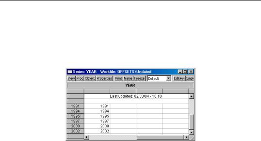
A few examples will help to illustrate the basic concepts. Suppose for example, that we have an irregular dated annual workfile with observations for the years “1991”, “1994”, “1995”, “1997”, “2000”, and “2002”:
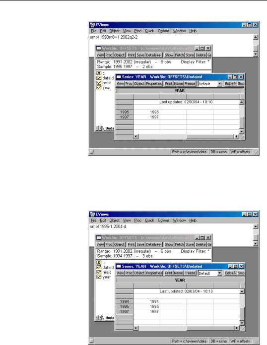
The sample statement:
smpl 1993m8+1 2002q2-2
is processed in several steps. First, the date “1993m8” is rounded to the previous regular frequency date, “1993”, and the date “2002q2” is rounded up to the last instance of the regular frequency date “2002”; thus, we have the equivalent sample statement:
smpl 1993+1 2002-2
Next, we find the base observations in the workfile corresponding to the base sample pair (“1993 2002”). The “1994” and the “2002” observations are the earliest and latest, respectively, that fall in the range.
102—Chapter 5. Basic Data Handling
Lastly, we apply the offsets to the remaining observations.
The offsets for the start and end will drop one observation (“1994”) from the beginning and two observations (“2002” and “2000”) from the end of the sample, leaving two observations (“1995”, “1997”) in the sample.
Consider instead the sample statement:
smpl 1995-1 2004-4
In this case, no rounding is necessary since the dates are specified in the workfile frequency.
For the start of the date pair, we note that the observation for “1995” corresponds to the start date. Computing the offset “-1” simply adds the “1994” observation.
For the end of the date pair, we note that “2004” is beyond the last observation in the workfile, “2002”. We begin by computing offsets to “2004” using the regular fre-