

- •Table of Contents
- •What’s New in EViews 5.0
- •What’s New in 5.0
- •Compatibility Notes
- •EViews 5.1 Update Overview
- •Overview of EViews 5.1 New Features
- •Preface
- •Part I. EViews Fundamentals
- •Chapter 1. Introduction
- •What is EViews?
- •Installing and Running EViews
- •Windows Basics
- •The EViews Window
- •Closing EViews
- •Where to Go For Help
- •Chapter 2. A Demonstration
- •Getting Data into EViews
- •Examining the Data
- •Estimating a Regression Model
- •Specification and Hypothesis Tests
- •Modifying the Equation
- •Forecasting from an Estimated Equation
- •Additional Testing
- •Chapter 3. Workfile Basics
- •What is a Workfile?
- •Creating a Workfile
- •The Workfile Window
- •Saving a Workfile
- •Loading a Workfile
- •Multi-page Workfiles
- •Addendum: File Dialog Features
- •Chapter 4. Object Basics
- •What is an Object?
- •Basic Object Operations
- •The Object Window
- •Working with Objects
- •Chapter 5. Basic Data Handling
- •Data Objects
- •Samples
- •Sample Objects
- •Importing Data
- •Exporting Data
- •Frequency Conversion
- •Importing ASCII Text Files
- •Chapter 6. Working with Data
- •Numeric Expressions
- •Series
- •Auto-series
- •Groups
- •Scalars
- •Chapter 7. Working with Data (Advanced)
- •Auto-Updating Series
- •Alpha Series
- •Date Series
- •Value Maps
- •Chapter 8. Series Links
- •Basic Link Concepts
- •Creating a Link
- •Working with Links
- •Chapter 9. Advanced Workfiles
- •Structuring a Workfile
- •Resizing a Workfile
- •Appending to a Workfile
- •Contracting a Workfile
- •Copying from a Workfile
- •Reshaping a Workfile
- •Sorting a Workfile
- •Exporting from a Workfile
- •Chapter 10. EViews Databases
- •Database Overview
- •Database Basics
- •Working with Objects in Databases
- •Database Auto-Series
- •The Database Registry
- •Querying the Database
- •Object Aliases and Illegal Names
- •Maintaining the Database
- •Foreign Format Databases
- •Working with DRIPro Links
- •Part II. Basic Data Analysis
- •Chapter 11. Series
- •Series Views Overview
- •Spreadsheet and Graph Views
- •Descriptive Statistics
- •Tests for Descriptive Stats
- •Distribution Graphs
- •One-Way Tabulation
- •Correlogram
- •Unit Root Test
- •BDS Test
- •Properties
- •Label
- •Series Procs Overview
- •Generate by Equation
- •Resample
- •Seasonal Adjustment
- •Exponential Smoothing
- •Hodrick-Prescott Filter
- •Frequency (Band-Pass) Filter
- •Chapter 12. Groups
- •Group Views Overview
- •Group Members
- •Spreadsheet
- •Dated Data Table
- •Graphs
- •Multiple Graphs
- •Descriptive Statistics
- •Tests of Equality
- •N-Way Tabulation
- •Principal Components
- •Correlations, Covariances, and Correlograms
- •Cross Correlations and Correlograms
- •Cointegration Test
- •Unit Root Test
- •Granger Causality
- •Label
- •Group Procedures Overview
- •Chapter 13. Statistical Graphs from Series and Groups
- •Distribution Graphs of Series
- •Scatter Diagrams with Fit Lines
- •Boxplots
- •Chapter 14. Graphs, Tables, and Text Objects
- •Creating Graphs
- •Modifying Graphs
- •Multiple Graphs
- •Printing Graphs
- •Copying Graphs to the Clipboard
- •Saving Graphs to a File
- •Graph Commands
- •Creating Tables
- •Table Basics
- •Basic Table Customization
- •Customizing Table Cells
- •Copying Tables to the Clipboard
- •Saving Tables to a File
- •Table Commands
- •Text Objects
- •Part III. Basic Single Equation Analysis
- •Chapter 15. Basic Regression
- •Equation Objects
- •Specifying an Equation in EViews
- •Estimating an Equation in EViews
- •Equation Output
- •Working with Equations
- •Estimation Problems
- •Chapter 16. Additional Regression Methods
- •Special Equation Terms
- •Weighted Least Squares
- •Heteroskedasticity and Autocorrelation Consistent Covariances
- •Two-stage Least Squares
- •Nonlinear Least Squares
- •Generalized Method of Moments (GMM)
- •Chapter 17. Time Series Regression
- •Serial Correlation Theory
- •Testing for Serial Correlation
- •Estimating AR Models
- •ARIMA Theory
- •Estimating ARIMA Models
- •ARMA Equation Diagnostics
- •Nonstationary Time Series
- •Unit Root Tests
- •Panel Unit Root Tests
- •Chapter 18. Forecasting from an Equation
- •Forecasting from Equations in EViews
- •An Illustration
- •Forecast Basics
- •Forecasting with ARMA Errors
- •Forecasting from Equations with Expressions
- •Forecasting with Expression and PDL Specifications
- •Chapter 19. Specification and Diagnostic Tests
- •Background
- •Coefficient Tests
- •Residual Tests
- •Specification and Stability Tests
- •Applications
- •Part IV. Advanced Single Equation Analysis
- •Chapter 20. ARCH and GARCH Estimation
- •Basic ARCH Specifications
- •Estimating ARCH Models in EViews
- •Working with ARCH Models
- •Additional ARCH Models
- •Examples
- •Binary Dependent Variable Models
- •Estimating Binary Models in EViews
- •Procedures for Binary Equations
- •Ordered Dependent Variable Models
- •Estimating Ordered Models in EViews
- •Views of Ordered Equations
- •Procedures for Ordered Equations
- •Censored Regression Models
- •Estimating Censored Models in EViews
- •Procedures for Censored Equations
- •Truncated Regression Models
- •Procedures for Truncated Equations
- •Count Models
- •Views of Count Models
- •Procedures for Count Models
- •Demonstrations
- •Technical Notes
- •Chapter 22. The Log Likelihood (LogL) Object
- •Overview
- •Specification
- •Estimation
- •LogL Views
- •LogL Procs
- •Troubleshooting
- •Limitations
- •Examples
- •Part V. Multiple Equation Analysis
- •Chapter 23. System Estimation
- •Background
- •System Estimation Methods
- •How to Create and Specify a System
- •Working With Systems
- •Technical Discussion
- •Vector Autoregressions (VARs)
- •Estimating a VAR in EViews
- •VAR Estimation Output
- •Views and Procs of a VAR
- •Structural (Identified) VARs
- •Cointegration Test
- •Vector Error Correction (VEC) Models
- •A Note on Version Compatibility
- •Chapter 25. State Space Models and the Kalman Filter
- •Background
- •Specifying a State Space Model in EViews
- •Working with the State Space
- •Converting from Version 3 Sspace
- •Technical Discussion
- •Chapter 26. Models
- •Overview
- •An Example Model
- •Building a Model
- •Working with the Model Structure
- •Specifying Scenarios
- •Using Add Factors
- •Solving the Model
- •Working with the Model Data
- •Part VI. Panel and Pooled Data
- •Chapter 27. Pooled Time Series, Cross-Section Data
- •The Pool Workfile
- •The Pool Object
- •Pooled Data
- •Setting up a Pool Workfile
- •Working with Pooled Data
- •Pooled Estimation
- •Chapter 28. Working with Panel Data
- •Structuring a Panel Workfile
- •Panel Workfile Display
- •Panel Workfile Information
- •Working with Panel Data
- •Basic Panel Analysis
- •Chapter 29. Panel Estimation
- •Estimating a Panel Equation
- •Panel Estimation Examples
- •Panel Equation Testing
- •Estimation Background
- •Appendix A. Global Options
- •The Options Menu
- •Print Setup
- •Appendix B. Wildcards
- •Wildcard Expressions
- •Using Wildcard Expressions
- •Source and Destination Patterns
- •Resolving Ambiguities
- •Wildcard versus Pool Identifier
- •Appendix C. Estimation and Solution Options
- •Setting Estimation Options
- •Optimization Algorithms
- •Nonlinear Equation Solution Methods
- •Appendix D. Gradients and Derivatives
- •Gradients
- •Derivatives
- •Appendix E. Information Criteria
- •Definitions
- •Using Information Criteria as a Guide to Model Selection
- •References
- •Index
- •Symbols
- •.DB? files 266
- •.EDB file 262
- •.RTF file 437
- •.WF1 file 62
- •@obsnum
- •Panel
- •@unmaptxt 174
- •~, in backup file name 62, 939
- •Numerics
- •3sls (three-stage least squares) 697, 716
- •Abort key 21
- •ARIMA models 501
- •ASCII
- •file export 115
- •ASCII file
- •See also Unit root tests.
- •Auto-search
- •Auto-series
- •in groups 144
- •Auto-updating series
- •and databases 152
- •Backcast
- •Berndt-Hall-Hall-Hausman (BHHH). See Optimization algorithms.
- •Bias proportion 554
- •fitted index 634
- •Binning option
- •classifications 313, 382
- •Boxplots 409
- •By-group statistics 312, 886, 893
- •coef vector 444
- •Causality
- •Granger's test 389
- •scale factor 649
- •Census X11
- •Census X12 337
- •Chi-square
- •Cholesky factor
- •Classification table
- •Close
- •Coef (coefficient vector)
- •default 444
- •Coefficient
- •Comparison operators
- •Conditional standard deviation
- •graph 610
- •Confidence interval
- •Constant
- •Copy
- •data cut-and-paste 107
- •table to clipboard 437
- •Covariance matrix
- •HAC (Newey-West) 473
- •heteroskedasticity consistent of estimated coefficients 472
- •Create
- •Cross-equation
- •Tukey option 393
- •CUSUM
- •sum of recursive residuals test 589
- •sum of recursive squared residuals test 590
- •Data
- •Database
- •link options 303
- •using auto-updating series with 152
- •Dates
- •Default
- •database 24, 266
- •set directory 71
- •Dependent variable
- •Description
- •Descriptive statistics
- •by group 312
- •group 379
- •individual samples (group) 379
- •Display format
- •Display name
- •Distribution
- •Dummy variables
- •for regression 452
- •lagged dependent variable 495
- •Dynamic forecasting 556
- •Edit
- •See also Unit root tests.
- •Equation
- •create 443
- •store 458
- •Estimation
- •EViews
- •Excel file
- •Excel files
- •Expectation-prediction table
- •Expected dependent variable
- •double 352
- •Export data 114
- •Extreme value
- •binary model 624
- •Fetch
- •File
- •save table to 438
- •Files
- •Fitted index
- •Fitted values
- •Font options
- •Fonts
- •Forecast
- •evaluation 553
- •Foreign data
- •Formula
- •forecast 561
- •Freq
- •DRI database 303
- •F-test
- •for variance equality 321
- •Full information maximum likelihood 698
- •GARCH 601
- •ARCH-M model 603
- •variance factor 668
- •system 716
- •Goodness-of-fit
- •Gradients 963
- •Graph
- •remove elements 423
- •Groups
- •display format 94
- •Groupwise heteroskedasticity 380
- •Help
- •Heteroskedasticity and autocorrelation consistent covariance (HAC) 473
- •History
- •Holt-Winters
- •Hypothesis tests
- •F-test 321
- •Identification
- •Identity
- •Import
- •Import data
- •See also VAR.
- •Index
- •Insert
- •Instruments 474
- •Iteration
- •Iteration option 953
- •in nonlinear least squares 483
- •J-statistic 491
- •J-test 596
- •Kernel
- •bivariate fit 405
- •choice in HAC weighting 704, 718
- •Kernel function
- •Keyboard
- •Kwiatkowski, Phillips, Schmidt, and Shin test 525
- •Label 82
- •Last_update
- •Last_write
- •Latent variable
- •Lead
- •make covariance matrix 643
- •List
- •LM test
- •ARCH 582
- •for binary models 622
- •LOWESS. See also LOESS
- •in ARIMA models 501
- •Mean absolute error 553
- •Metafile
- •Micro TSP
- •recoding 137
- •Models
- •add factors 777, 802
- •solving 804
- •Mouse 18
- •Multicollinearity 460
- •Name
- •Newey-West
- •Nonlinear coefficient restriction
- •Wald test 575
- •weighted two stage 486
- •Normal distribution
- •Numbers
- •chi-square tests 383
- •Object 73
- •Open
- •Option setting
- •Option settings
- •Or operator 98, 133
- •Ordinary residual
- •Panel
- •irregular 214
- •unit root tests 530
- •Paste 83
- •PcGive data 293
- •Polynomial distributed lag
- •Pool
- •Pool (object)
- •PostScript
- •Prediction table
- •Principal components 385
- •Program
- •p-value 569
- •for coefficient t-statistic 450
- •Quiet mode 939
- •RATS data
- •Read 832
- •CUSUM 589
- •Regression
- •Relational operators
- •Remarks
- •database 287
- •Residuals
- •Resize
- •Results
- •RichText Format
- •Robust standard errors
- •Robustness iterations
- •for regression 451
- •with AR specification 500
- •workfile 95
- •Save
- •Seasonal
- •Seasonal graphs 310
- •Select
- •single item 20
- •Serial correlation
- •theory 493
- •Series
- •Smoothing
- •Solve
- •Source
- •Specification test
- •Spreadsheet
- •Standard error
- •Standard error
- •binary models 634
- •Start
- •Starting values
- •Summary statistics
- •for regression variables 451
- •System
- •Table 429
- •font 434
- •Tabulation
- •Template 424
- •Tests. See also Hypothesis tests, Specification test and Goodness of fit.
- •Text file
- •open as workfile 54
- •Type
- •field in database query 282
- •Units
- •Update
- •Valmap
- •find label for value 173
- •find numeric value for label 174
- •Value maps 163
- •estimating 749
- •View
- •Wald test 572
- •nonlinear restriction 575
- •Watson test 323
- •Weighting matrix
- •heteroskedasticity and autocorrelation consistent (HAC) 718
- •kernel options 718
- •White
- •Window
- •Workfile
- •storage defaults 940
- •Write 844
- •XY line
- •Yates' continuity correction 321

Multiple Graphs—425
line, symbol, and filled area settings. Once applied, these changes cannot be undone automatically.
In contrast to the basic graph settings which are always updated when you click on Apply, the impact on the characteristics of existing text, line, and shade objects in the graph (“Added Text, Line, and Shade Attribute Defaults” on page 421) is controlled by the choices on the right-hand side of the dialog. There are three possibilities:
•Keep old settings – instructs EViews to use the text, line, and shade attributes in the template or template graph only for the purpose of updating the default settings in the graph. If you select this option and select Apply, subsequently added text, line, and shades will use the updated settings, but existing objects will retain their existing characterisitcs.
•Apply template settings to existing text & line/shade objects – will update both the settings for existing text, line, and shade objects, and the defaults used for newly added objects.
•Replace text & line/shade objects with those of the template graph – will first remove any added text label, line, or shading objects in the existing graph, and then copy to the graph any such objects in the template.
Setting Global Defaults
You may change the default settings for any of these options by selecting Options/Graphics Defaults... from the main EViews menu. Any new graph views or objects will use the graphic options as the default settings.
Multiple Graphs
Some views are made up of multiple graphs. Like single graph views, these may be turned into graph objects by freezing. For example, the impulse response view of a VAR can display multiple graphs in a single view.
You may also create a graph object containing multiple graphs by combining existing named graph objects. Simply select the desired graphs and then double click on any one of the highlighted names. An alternative method of combining graphs is to select Quick/ Show… and enter the names of the graphs.
There are two ways to work with a multiple graph. You may change the settings for the multiple graph as a whole, or you may work with an individual graph component of the multiple graph.

426—Chapter 14. Graphs, Tables, and Text Objects
Working With Multiple Graphs
EViews makes it easy to work with all of the graphs in a multiple graph. Simply select Proc from the graph menu and EViews will display a menu prompting you for additional choices.
These menu items set options that apply to all graphs in the graph object.
•To set a common graph attribute to all graphs, select Options on all graphs…. Alternately, you may click anywhere in the background area of the multiple graph. After selecting the desired options, check the Apply page to all graphs checkbox at the bottom of the tab.
•While each single graph in a multiple graph can be freely positioned by dragging the graph, you may wish to globally align graphs in columns and control the overall spacing between graphs. To globally position your graphs, select Position and align graphs...
•If all of your graphs share a common axis, you can draw lines or add shading to each graph in the object, by selecting Add shading to all graphs….
•Selecting Add text… allows you to annotate your multiple graph. Note that adding an item to the multiple graph differs from adding it to an individual graph since it will not move with the individual graph.
•Selecting Template... allows you to apply a template graph to each individual graph in your multiple graph or to reset the graph to use the global defaults.
•Save graph to disk... brings up the File Save dialog, as described in “Saving Graphs to a File” on page 429.
There is a shortcut method if you merely wish to set the options for all of your graphs. Simply double click anywhere in the background area of your graph, and EViews will open the multiple Graph Options dialog.
Working with Individual Graphs
You may change the options for an individual graph in the usual fashion by double clicking on the graph to display the options dialog.

Printing Graphs—427
You can also perform various operations on individual graphs. Click on the graph and EViews will confirm the selection by surrounding the individual graph with a blue border. Select Proc or right mouse click to display a menu that allows you to set options, add text or shading, apply a template or reset options to the global defaults, to remove the selected graph, or to save the graph to disk. Deleting the selected graph can also be performed
by pressing the Remove button on the graph toolbar or the Delete key.
In addition, you can place each individual graph at an arbitrary position by simply dragging the individual graph to the desired location.
An Example
Here is an example of an annotated and customized combined graph created in EViews and copied-and-pasted into a word processor:
LOESS fit
|
0.04 |
|
|
|
|
|
|
0.03 |
|
|
|
|
|
inflation |
0.02 |
|
|
|
|
|
0.01 |
|
|
|
|
|
|
|
|
|
|
|
|
|
wage |
0.00 |
|
|
|
|
|
|
|
|
|
|
|
|
|
-0.01 |
|
|
|
|
|
|
0.02 |
0.04 |
0.06 |
0.08 |
0.10 |
0.12 |
Forecast intervals (95%) of M1
1300
1200
1100 |
actual M1 |
|
|
1000 |
|
900 |
|
800 |
|
1990 1991 1992 1993 1994 1995
civilian unemployment rate
See “Copying Tables to the Clipboard” on page 437 for additional discussion of exporting graphs via copy-and-paste.
Printing Graphs
Clicking on the Print button on the graph view or graph object window toolbar will open the Print dialog, allowing you to override the various global settings for graph printing.
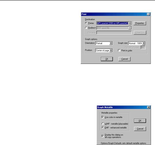
428—Chapter 14. Graphs, Tables, and Text Objects
Most of the options are self-explanatory. If you wish to print your graph in color using your color printer, make certain that the Print in color box is checked. Conversely, if you are printing to a black and white printer, you should make certain that this box is not checked so that EViews will substitute line patterns for colors. See “Print Setup” on page 943 for additional details.
Copying Graphs to the Clipboard
You can incorporate an EViews graph view or object directly into a document in your Windows word processor. First, you should activate the object window containing the graph you wish to move by clicking anywhere in the window (the titlebar of the object window should change to a bright color). Then click on Edit/Copy on the EViews main menu; the Graph Metafile dialog box appears. The default settings in this dialog are taken from the global defaults.
You can copy the graph to the Windows clipboard in Windows metafile (WMF) or enhanced metafile (EMF) formats. You can request that the graph be in color and that its lines be in bold. We recommend that you copy graphs in black-and-white unless you will be printing to a color printer.
Once you copy a graph to the clipboard, you may then switch to your word processor and paste the graph into your document. Standard programs such
as Microsoft Word will give you a graph which can be sized, positioned, and modified within the program. You can also paste graphs into drawing programs, and make further modifications before pasting into your word processor or other software.
You may choose to hide this copy dialog for subsequent operations by unchecking the Display this dialog... box. Copying will then always use the default settings, without prompting. If you wish to change the default settings, or to turn on or off the display of the copy dialog, you may go to the Exporting tab of the global Graph options (Options/Graphics Defaults...).