

- •Table of Contents
- •What’s New in EViews 5.0
- •What’s New in 5.0
- •Compatibility Notes
- •EViews 5.1 Update Overview
- •Overview of EViews 5.1 New Features
- •Preface
- •Part I. EViews Fundamentals
- •Chapter 1. Introduction
- •What is EViews?
- •Installing and Running EViews
- •Windows Basics
- •The EViews Window
- •Closing EViews
- •Where to Go For Help
- •Chapter 2. A Demonstration
- •Getting Data into EViews
- •Examining the Data
- •Estimating a Regression Model
- •Specification and Hypothesis Tests
- •Modifying the Equation
- •Forecasting from an Estimated Equation
- •Additional Testing
- •Chapter 3. Workfile Basics
- •What is a Workfile?
- •Creating a Workfile
- •The Workfile Window
- •Saving a Workfile
- •Loading a Workfile
- •Multi-page Workfiles
- •Addendum: File Dialog Features
- •Chapter 4. Object Basics
- •What is an Object?
- •Basic Object Operations
- •The Object Window
- •Working with Objects
- •Chapter 5. Basic Data Handling
- •Data Objects
- •Samples
- •Sample Objects
- •Importing Data
- •Exporting Data
- •Frequency Conversion
- •Importing ASCII Text Files
- •Chapter 6. Working with Data
- •Numeric Expressions
- •Series
- •Auto-series
- •Groups
- •Scalars
- •Chapter 7. Working with Data (Advanced)
- •Auto-Updating Series
- •Alpha Series
- •Date Series
- •Value Maps
- •Chapter 8. Series Links
- •Basic Link Concepts
- •Creating a Link
- •Working with Links
- •Chapter 9. Advanced Workfiles
- •Structuring a Workfile
- •Resizing a Workfile
- •Appending to a Workfile
- •Contracting a Workfile
- •Copying from a Workfile
- •Reshaping a Workfile
- •Sorting a Workfile
- •Exporting from a Workfile
- •Chapter 10. EViews Databases
- •Database Overview
- •Database Basics
- •Working with Objects in Databases
- •Database Auto-Series
- •The Database Registry
- •Querying the Database
- •Object Aliases and Illegal Names
- •Maintaining the Database
- •Foreign Format Databases
- •Working with DRIPro Links
- •Part II. Basic Data Analysis
- •Chapter 11. Series
- •Series Views Overview
- •Spreadsheet and Graph Views
- •Descriptive Statistics
- •Tests for Descriptive Stats
- •Distribution Graphs
- •One-Way Tabulation
- •Correlogram
- •Unit Root Test
- •BDS Test
- •Properties
- •Label
- •Series Procs Overview
- •Generate by Equation
- •Resample
- •Seasonal Adjustment
- •Exponential Smoothing
- •Hodrick-Prescott Filter
- •Frequency (Band-Pass) Filter
- •Chapter 12. Groups
- •Group Views Overview
- •Group Members
- •Spreadsheet
- •Dated Data Table
- •Graphs
- •Multiple Graphs
- •Descriptive Statistics
- •Tests of Equality
- •N-Way Tabulation
- •Principal Components
- •Correlations, Covariances, and Correlograms
- •Cross Correlations and Correlograms
- •Cointegration Test
- •Unit Root Test
- •Granger Causality
- •Label
- •Group Procedures Overview
- •Chapter 13. Statistical Graphs from Series and Groups
- •Distribution Graphs of Series
- •Scatter Diagrams with Fit Lines
- •Boxplots
- •Chapter 14. Graphs, Tables, and Text Objects
- •Creating Graphs
- •Modifying Graphs
- •Multiple Graphs
- •Printing Graphs
- •Copying Graphs to the Clipboard
- •Saving Graphs to a File
- •Graph Commands
- •Creating Tables
- •Table Basics
- •Basic Table Customization
- •Customizing Table Cells
- •Copying Tables to the Clipboard
- •Saving Tables to a File
- •Table Commands
- •Text Objects
- •Part III. Basic Single Equation Analysis
- •Chapter 15. Basic Regression
- •Equation Objects
- •Specifying an Equation in EViews
- •Estimating an Equation in EViews
- •Equation Output
- •Working with Equations
- •Estimation Problems
- •Chapter 16. Additional Regression Methods
- •Special Equation Terms
- •Weighted Least Squares
- •Heteroskedasticity and Autocorrelation Consistent Covariances
- •Two-stage Least Squares
- •Nonlinear Least Squares
- •Generalized Method of Moments (GMM)
- •Chapter 17. Time Series Regression
- •Serial Correlation Theory
- •Testing for Serial Correlation
- •Estimating AR Models
- •ARIMA Theory
- •Estimating ARIMA Models
- •ARMA Equation Diagnostics
- •Nonstationary Time Series
- •Unit Root Tests
- •Panel Unit Root Tests
- •Chapter 18. Forecasting from an Equation
- •Forecasting from Equations in EViews
- •An Illustration
- •Forecast Basics
- •Forecasting with ARMA Errors
- •Forecasting from Equations with Expressions
- •Forecasting with Expression and PDL Specifications
- •Chapter 19. Specification and Diagnostic Tests
- •Background
- •Coefficient Tests
- •Residual Tests
- •Specification and Stability Tests
- •Applications
- •Part IV. Advanced Single Equation Analysis
- •Chapter 20. ARCH and GARCH Estimation
- •Basic ARCH Specifications
- •Estimating ARCH Models in EViews
- •Working with ARCH Models
- •Additional ARCH Models
- •Examples
- •Binary Dependent Variable Models
- •Estimating Binary Models in EViews
- •Procedures for Binary Equations
- •Ordered Dependent Variable Models
- •Estimating Ordered Models in EViews
- •Views of Ordered Equations
- •Procedures for Ordered Equations
- •Censored Regression Models
- •Estimating Censored Models in EViews
- •Procedures for Censored Equations
- •Truncated Regression Models
- •Procedures for Truncated Equations
- •Count Models
- •Views of Count Models
- •Procedures for Count Models
- •Demonstrations
- •Technical Notes
- •Chapter 22. The Log Likelihood (LogL) Object
- •Overview
- •Specification
- •Estimation
- •LogL Views
- •LogL Procs
- •Troubleshooting
- •Limitations
- •Examples
- •Part V. Multiple Equation Analysis
- •Chapter 23. System Estimation
- •Background
- •System Estimation Methods
- •How to Create and Specify a System
- •Working With Systems
- •Technical Discussion
- •Vector Autoregressions (VARs)
- •Estimating a VAR in EViews
- •VAR Estimation Output
- •Views and Procs of a VAR
- •Structural (Identified) VARs
- •Cointegration Test
- •Vector Error Correction (VEC) Models
- •A Note on Version Compatibility
- •Chapter 25. State Space Models and the Kalman Filter
- •Background
- •Specifying a State Space Model in EViews
- •Working with the State Space
- •Converting from Version 3 Sspace
- •Technical Discussion
- •Chapter 26. Models
- •Overview
- •An Example Model
- •Building a Model
- •Working with the Model Structure
- •Specifying Scenarios
- •Using Add Factors
- •Solving the Model
- •Working with the Model Data
- •Part VI. Panel and Pooled Data
- •Chapter 27. Pooled Time Series, Cross-Section Data
- •The Pool Workfile
- •The Pool Object
- •Pooled Data
- •Setting up a Pool Workfile
- •Working with Pooled Data
- •Pooled Estimation
- •Chapter 28. Working with Panel Data
- •Structuring a Panel Workfile
- •Panel Workfile Display
- •Panel Workfile Information
- •Working with Panel Data
- •Basic Panel Analysis
- •Chapter 29. Panel Estimation
- •Estimating a Panel Equation
- •Panel Estimation Examples
- •Panel Equation Testing
- •Estimation Background
- •Appendix A. Global Options
- •The Options Menu
- •Print Setup
- •Appendix B. Wildcards
- •Wildcard Expressions
- •Using Wildcard Expressions
- •Source and Destination Patterns
- •Resolving Ambiguities
- •Wildcard versus Pool Identifier
- •Appendix C. Estimation and Solution Options
- •Setting Estimation Options
- •Optimization Algorithms
- •Nonlinear Equation Solution Methods
- •Appendix D. Gradients and Derivatives
- •Gradients
- •Derivatives
- •Appendix E. Information Criteria
- •Definitions
- •Using Information Criteria as a Guide to Model Selection
- •References
- •Index
- •Symbols
- •.DB? files 266
- •.EDB file 262
- •.RTF file 437
- •.WF1 file 62
- •@obsnum
- •Panel
- •@unmaptxt 174
- •~, in backup file name 62, 939
- •Numerics
- •3sls (three-stage least squares) 697, 716
- •Abort key 21
- •ARIMA models 501
- •ASCII
- •file export 115
- •ASCII file
- •See also Unit root tests.
- •Auto-search
- •Auto-series
- •in groups 144
- •Auto-updating series
- •and databases 152
- •Backcast
- •Berndt-Hall-Hall-Hausman (BHHH). See Optimization algorithms.
- •Bias proportion 554
- •fitted index 634
- •Binning option
- •classifications 313, 382
- •Boxplots 409
- •By-group statistics 312, 886, 893
- •coef vector 444
- •Causality
- •Granger's test 389
- •scale factor 649
- •Census X11
- •Census X12 337
- •Chi-square
- •Cholesky factor
- •Classification table
- •Close
- •Coef (coefficient vector)
- •default 444
- •Coefficient
- •Comparison operators
- •Conditional standard deviation
- •graph 610
- •Confidence interval
- •Constant
- •Copy
- •data cut-and-paste 107
- •table to clipboard 437
- •Covariance matrix
- •HAC (Newey-West) 473
- •heteroskedasticity consistent of estimated coefficients 472
- •Create
- •Cross-equation
- •Tukey option 393
- •CUSUM
- •sum of recursive residuals test 589
- •sum of recursive squared residuals test 590
- •Data
- •Database
- •link options 303
- •using auto-updating series with 152
- •Dates
- •Default
- •database 24, 266
- •set directory 71
- •Dependent variable
- •Description
- •Descriptive statistics
- •by group 312
- •group 379
- •individual samples (group) 379
- •Display format
- •Display name
- •Distribution
- •Dummy variables
- •for regression 452
- •lagged dependent variable 495
- •Dynamic forecasting 556
- •Edit
- •See also Unit root tests.
- •Equation
- •create 443
- •store 458
- •Estimation
- •EViews
- •Excel file
- •Excel files
- •Expectation-prediction table
- •Expected dependent variable
- •double 352
- •Export data 114
- •Extreme value
- •binary model 624
- •Fetch
- •File
- •save table to 438
- •Files
- •Fitted index
- •Fitted values
- •Font options
- •Fonts
- •Forecast
- •evaluation 553
- •Foreign data
- •Formula
- •forecast 561
- •Freq
- •DRI database 303
- •F-test
- •for variance equality 321
- •Full information maximum likelihood 698
- •GARCH 601
- •ARCH-M model 603
- •variance factor 668
- •system 716
- •Goodness-of-fit
- •Gradients 963
- •Graph
- •remove elements 423
- •Groups
- •display format 94
- •Groupwise heteroskedasticity 380
- •Help
- •Heteroskedasticity and autocorrelation consistent covariance (HAC) 473
- •History
- •Holt-Winters
- •Hypothesis tests
- •F-test 321
- •Identification
- •Identity
- •Import
- •Import data
- •See also VAR.
- •Index
- •Insert
- •Instruments 474
- •Iteration
- •Iteration option 953
- •in nonlinear least squares 483
- •J-statistic 491
- •J-test 596
- •Kernel
- •bivariate fit 405
- •choice in HAC weighting 704, 718
- •Kernel function
- •Keyboard
- •Kwiatkowski, Phillips, Schmidt, and Shin test 525
- •Label 82
- •Last_update
- •Last_write
- •Latent variable
- •Lead
- •make covariance matrix 643
- •List
- •LM test
- •ARCH 582
- •for binary models 622
- •LOWESS. See also LOESS
- •in ARIMA models 501
- •Mean absolute error 553
- •Metafile
- •Micro TSP
- •recoding 137
- •Models
- •add factors 777, 802
- •solving 804
- •Mouse 18
- •Multicollinearity 460
- •Name
- •Newey-West
- •Nonlinear coefficient restriction
- •Wald test 575
- •weighted two stage 486
- •Normal distribution
- •Numbers
- •chi-square tests 383
- •Object 73
- •Open
- •Option setting
- •Option settings
- •Or operator 98, 133
- •Ordinary residual
- •Panel
- •irregular 214
- •unit root tests 530
- •Paste 83
- •PcGive data 293
- •Polynomial distributed lag
- •Pool
- •Pool (object)
- •PostScript
- •Prediction table
- •Principal components 385
- •Program
- •p-value 569
- •for coefficient t-statistic 450
- •Quiet mode 939
- •RATS data
- •Read 832
- •CUSUM 589
- •Regression
- •Relational operators
- •Remarks
- •database 287
- •Residuals
- •Resize
- •Results
- •RichText Format
- •Robust standard errors
- •Robustness iterations
- •for regression 451
- •with AR specification 500
- •workfile 95
- •Save
- •Seasonal
- •Seasonal graphs 310
- •Select
- •single item 20
- •Serial correlation
- •theory 493
- •Series
- •Smoothing
- •Solve
- •Source
- •Specification test
- •Spreadsheet
- •Standard error
- •Standard error
- •binary models 634
- •Start
- •Starting values
- •Summary statistics
- •for regression variables 451
- •System
- •Table 429
- •font 434
- •Tabulation
- •Template 424
- •Tests. See also Hypothesis tests, Specification test and Goodness of fit.
- •Text file
- •open as workfile 54
- •Type
- •field in database query 282
- •Units
- •Update
- •Valmap
- •find label for value 173
- •find numeric value for label 174
- •Value maps 163
- •estimating 749
- •View
- •Wald test 572
- •nonlinear restriction 575
- •Watson test 323
- •Weighting matrix
- •heteroskedasticity and autocorrelation consistent (HAC) 718
- •kernel options 718
- •White
- •Window
- •Workfile
- •storage defaults 940
- •Write 844
- •XY line
- •Yates' continuity correction 321

Chapter 15. Basic Regression
Single equation regression is one of the most versatile and widely used statistical techniques. Here, we describe the use of basic regression techniques in EViews: specifying and estimating a regression model, performing simple diagnostic analysis, and using your estimation results in further analysis.
Subsequent chapters discuss testing and forecasting, as well as more advanced and specialized techniques such as weighted least squares, two-stage least squares (TSLS), nonlinear least squares, ARIMA/ARIMAX models, generalized method of moments (GMM), GARCH models, and qualitative and limited dependent variable models. These techniques and models all build upon the basic ideas presented in this chapter.
You will probably find it useful to own an econometrics textbook as a reference for the techniques discussed in this and subsequent documentation. Standard textbooks that we have found to be useful are listed below (in generally increasing order of difficulty):
•Pindyck and Rubinfeld (1991), Econometric Models and Economic Forecasts, 3rd edition.
•Johnston and DiNardo (1997), Econometric Methods, 4th Edition.
•Wooldridge (2000), Introductory Econometrics: A Modern Approach.
•Greene (1997), Econometric Analysis, 3rd Edition.
•Davidson and MacKinnon (1993), Estimation and Inference in Econometrics.
Where appropriate, we will also provide you with specialized references for specific topics.
Equation Objects
Single equation regression estimation in EViews is performed using the equation object. To create an equation object in EViews: select Object/New Object.../Equation or Quick/Estimate Equation… from the main menu, or simply type the keyword equation in the command window.
Next, you will specify your equation in the Equation Specification dialog box that appears, and select an estimation method. Below, we provide details on specifying equations in EViews. EViews will estimate the equation and display results in the equation window.
The estimation results are stored as part of the equation object so they can be accessed at any time. Simply open the object to display the summary results, or to access EViews tools for working with results from an equation object. For example, you can retrieve the sum-
444—Chapter 15. Basic Regression
of-squares from any equation, or you can use the estimated equation as part of a multiequation model.
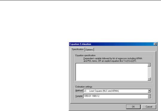
Specifying an Equation in EViews
When you create an equation object, a specification dialog box is displayed.
You need to specify three things in this dialog: the equation specification, the estimation method, and the sample to be used in estimation.
In the upper edit box, you can specify the equation: the dependent (left-hand side) and independent (right-hand side) variables and the functional form. There are two basic ways of specifying an equation: “by list” and “by formula” or “by expression”. The list method is easier but may
only be used with unrestricted linear specifications; the formula method is more general and must be used to specify nonlinear models or models with parametric restrictions.
Specifying an Equation by List
The simplest way to specify a linear equation is to provide a list of variables that you wish to use in the equation. First, include the name of the dependent variable or expression, followed by a list of explanatory variables. For example, to specify a linear consumption function, CS regressed on a constant and INC, type the following in the upper field of the
Equation Specification dialog:
cs c inc
Note the presence of the series name C in the list of regressors. This is a built-in EViews series that is used to specify a constant in a regression. EViews does not automatically include a constant in a regression so you must explicitly list the constant (or its equivalent) as a regressor. The internal series C does not appear in your workfile, and you may not use it outside of specifying an equation. If you need a series of ones, you can generate a new series, or use the number 1 as an auto-series.
You may have noticed that there is a pre-defined object C in your workfile. This is the default coefficient vector—when you specify an equation by listing variable names, EViews

Specifying an Equation in EViews—445
stores the estimated coefficients in this vector, in the order of appearance in the list. In the example above, the constant will be stored in C(1) and the coefficient on INC will be held in C(2).
Lagged series may be included in statistical operations using the same notation as in generating a new series with a formula—put the lag in parentheses after the name of the series. For example, the specification:
cs cs(-1) c inc
tells EViews to regress CS on its own lagged value, a constant, and INC. The coefficient for lagged CS will be placed in C(1), the coefficient for the constant is C(2), and the coefficient of INC is C(3).
You can include a consecutive range of lagged series by using the word “to” between the lags. For example:
cs c cs(-1 to -4) inc
regresses CS on a constant, CS(-1), CS(-2), CS(-3), CS(-4), and INC. If you don't include the first lag, it is taken to be zero. For example:
cs c inc(to -2) inc(-4)
regresses CS on a constant, INC, INC(-1), INC(-2), and INC(-4).
You may include auto-series in the list of variables. If the auto-series expressions contain spaces, they should be enclosed in parentheses. For example:
log(cs) c log(cs(-1)) ((inc+inc(-1)) / 2)
specifies a regression of the natural logarithm of CS on a constant, its own lagged value, and a two period moving average of INC.
Typing the list of series may be cumbersome, especially if you are working with many regressors. If you wish, EViews can create the specification list for you. First, highlight the dependent variable in the workfile window by single clicking on the entry. Next, CTRLclick on each of the explanatory variables to highlight them as well. When you are done selecting all of your variables, double click on any of the highlighted series, and select
Open/Equation…, or right click and select Open/as Equation.... The Equation Specification dialog box should appear with the names entered in the specification field. The constant C is automatically included in this list; you must delete the C if you do not wish to include the constant.

446—Chapter 15. Basic Regression
Specifying an Equation by Formula
You will need to specify your equation using a formula when the list method is not general enough for your specification. Many, but not all, estimation methods allow you to specify your equation using a formula.
An equation formula in EViews is a mathematical expression involving regressors and coefficients. To specify an equation using a formula, simply enter the expression in the dialog in place of the list of variables. EViews will add an implicit additive disturbance to this equation and will estimate the parameters of the model using least squares.
When you specify an equation by list, EViews converts this into an equivalent equation formula. For example, the list,
log(cs) c log(cs(-1)) log(inc)
is interpreted by EViews as:
log(cs) = c(1) + c(2)*log(cs(-1)) + c(3)*log(inc)
Equations do not have to have a dependent variable followed by an equal sign and then an expression. The “=” sign can be anywhere in the formula, as in:
log(urate) - c(1)*dmr = c(2) |
|
The residuals for this equation are given by: |
|
= log ( urate) − c( 1) dmr − c( 2 ) . |
(15.1) |
EViews will minimize the sum-of-squares of these residuals.
If you wish, you can specify an equation as a simple expression, without a dependent variable and an equal sign. If there is no equal sign, EViews assumes that the entire expression is the disturbance term. For example, if you specify an equation as:
c(1)*x + c(2)*y + 4*z
EViews will find the coefficient values that minimize the sum of squares of the given expression, in this case (C(1)*X+C(2)*Y+4*Z). While EViews will estimate an expression of this type, since there is no dependent variable, some regression statistics (e.g. R- squared) are not reported and the equation cannot be used for forecasting. This restriction also holds for any equation that includes coefficients to the left of the equal sign. For example, if you specify:
x + c(1)*y = c(2)*z
EViews finds the values of C(1) and C(2) that minimize the sum of squares of (X+C(1)*Y– C(2)*Z). The estimated coefficients will be identical to those from an equation specified using: