- •Table of Contents
- •What’s New in EViews 5.0
- •What’s New in 5.0
- •Compatibility Notes
- •EViews 5.1 Update Overview
- •Overview of EViews 5.1 New Features
- •Preface
- •Part I. EViews Fundamentals
- •Chapter 1. Introduction
- •What is EViews?
- •Installing and Running EViews
- •Windows Basics
- •The EViews Window
- •Closing EViews
- •Where to Go For Help
- •Chapter 2. A Demonstration
- •Getting Data into EViews
- •Examining the Data
- •Estimating a Regression Model
- •Specification and Hypothesis Tests
- •Modifying the Equation
- •Forecasting from an Estimated Equation
- •Additional Testing
- •Chapter 3. Workfile Basics
- •What is a Workfile?
- •Creating a Workfile
- •The Workfile Window
- •Saving a Workfile
- •Loading a Workfile
- •Multi-page Workfiles
- •Addendum: File Dialog Features
- •Chapter 4. Object Basics
- •What is an Object?
- •Basic Object Operations
- •The Object Window
- •Working with Objects
- •Chapter 5. Basic Data Handling
- •Data Objects
- •Samples
- •Sample Objects
- •Importing Data
- •Exporting Data
- •Frequency Conversion
- •Importing ASCII Text Files
- •Chapter 6. Working with Data
- •Numeric Expressions
- •Series
- •Auto-series
- •Groups
- •Scalars
- •Chapter 7. Working with Data (Advanced)
- •Auto-Updating Series
- •Alpha Series
- •Date Series
- •Value Maps
- •Chapter 8. Series Links
- •Basic Link Concepts
- •Creating a Link
- •Working with Links
- •Chapter 9. Advanced Workfiles
- •Structuring a Workfile
- •Resizing a Workfile
- •Appending to a Workfile
- •Contracting a Workfile
- •Copying from a Workfile
- •Reshaping a Workfile
- •Sorting a Workfile
- •Exporting from a Workfile
- •Chapter 10. EViews Databases
- •Database Overview
- •Database Basics
- •Working with Objects in Databases
- •Database Auto-Series
- •The Database Registry
- •Querying the Database
- •Object Aliases and Illegal Names
- •Maintaining the Database
- •Foreign Format Databases
- •Working with DRIPro Links
- •Part II. Basic Data Analysis
- •Chapter 11. Series
- •Series Views Overview
- •Spreadsheet and Graph Views
- •Descriptive Statistics
- •Tests for Descriptive Stats
- •Distribution Graphs
- •One-Way Tabulation
- •Correlogram
- •Unit Root Test
- •BDS Test
- •Properties
- •Label
- •Series Procs Overview
- •Generate by Equation
- •Resample
- •Seasonal Adjustment
- •Exponential Smoothing
- •Hodrick-Prescott Filter
- •Frequency (Band-Pass) Filter
- •Chapter 12. Groups
- •Group Views Overview
- •Group Members
- •Spreadsheet
- •Dated Data Table
- •Graphs
- •Multiple Graphs
- •Descriptive Statistics
- •Tests of Equality
- •N-Way Tabulation
- •Principal Components
- •Correlations, Covariances, and Correlograms
- •Cross Correlations and Correlograms
- •Cointegration Test
- •Unit Root Test
- •Granger Causality
- •Label
- •Group Procedures Overview
- •Chapter 13. Statistical Graphs from Series and Groups
- •Distribution Graphs of Series
- •Scatter Diagrams with Fit Lines
- •Boxplots
- •Chapter 14. Graphs, Tables, and Text Objects
- •Creating Graphs
- •Modifying Graphs
- •Multiple Graphs
- •Printing Graphs
- •Copying Graphs to the Clipboard
- •Saving Graphs to a File
- •Graph Commands
- •Creating Tables
- •Table Basics
- •Basic Table Customization
- •Customizing Table Cells
- •Copying Tables to the Clipboard
- •Saving Tables to a File
- •Table Commands
- •Text Objects
- •Part III. Basic Single Equation Analysis
- •Chapter 15. Basic Regression
- •Equation Objects
- •Specifying an Equation in EViews
- •Estimating an Equation in EViews
- •Equation Output
- •Working with Equations
- •Estimation Problems
- •Chapter 16. Additional Regression Methods
- •Special Equation Terms
- •Weighted Least Squares
- •Heteroskedasticity and Autocorrelation Consistent Covariances
- •Two-stage Least Squares
- •Nonlinear Least Squares
- •Generalized Method of Moments (GMM)
- •Chapter 17. Time Series Regression
- •Serial Correlation Theory
- •Testing for Serial Correlation
- •Estimating AR Models
- •ARIMA Theory
- •Estimating ARIMA Models
- •ARMA Equation Diagnostics
- •Nonstationary Time Series
- •Unit Root Tests
- •Panel Unit Root Tests
- •Chapter 18. Forecasting from an Equation
- •Forecasting from Equations in EViews
- •An Illustration
- •Forecast Basics
- •Forecasting with ARMA Errors
- •Forecasting from Equations with Expressions
- •Forecasting with Expression and PDL Specifications
- •Chapter 19. Specification and Diagnostic Tests
- •Background
- •Coefficient Tests
- •Residual Tests
- •Specification and Stability Tests
- •Applications
- •Part IV. Advanced Single Equation Analysis
- •Chapter 20. ARCH and GARCH Estimation
- •Basic ARCH Specifications
- •Estimating ARCH Models in EViews
- •Working with ARCH Models
- •Additional ARCH Models
- •Examples
- •Binary Dependent Variable Models
- •Estimating Binary Models in EViews
- •Procedures for Binary Equations
- •Ordered Dependent Variable Models
- •Estimating Ordered Models in EViews
- •Views of Ordered Equations
- •Procedures for Ordered Equations
- •Censored Regression Models
- •Estimating Censored Models in EViews
- •Procedures for Censored Equations
- •Truncated Regression Models
- •Procedures for Truncated Equations
- •Count Models
- •Views of Count Models
- •Procedures for Count Models
- •Demonstrations
- •Technical Notes
- •Chapter 22. The Log Likelihood (LogL) Object
- •Overview
- •Specification
- •Estimation
- •LogL Views
- •LogL Procs
- •Troubleshooting
- •Limitations
- •Examples
- •Part V. Multiple Equation Analysis
- •Chapter 23. System Estimation
- •Background
- •System Estimation Methods
- •How to Create and Specify a System
- •Working With Systems
- •Technical Discussion
- •Vector Autoregressions (VARs)
- •Estimating a VAR in EViews
- •VAR Estimation Output
- •Views and Procs of a VAR
- •Structural (Identified) VARs
- •Cointegration Test
- •Vector Error Correction (VEC) Models
- •A Note on Version Compatibility
- •Chapter 25. State Space Models and the Kalman Filter
- •Background
- •Specifying a State Space Model in EViews
- •Working with the State Space
- •Converting from Version 3 Sspace
- •Technical Discussion
- •Chapter 26. Models
- •Overview
- •An Example Model
- •Building a Model
- •Working with the Model Structure
- •Specifying Scenarios
- •Using Add Factors
- •Solving the Model
- •Working with the Model Data
- •Part VI. Panel and Pooled Data
- •Chapter 27. Pooled Time Series, Cross-Section Data
- •The Pool Workfile
- •The Pool Object
- •Pooled Data
- •Setting up a Pool Workfile
- •Working with Pooled Data
- •Pooled Estimation
- •Chapter 28. Working with Panel Data
- •Structuring a Panel Workfile
- •Panel Workfile Display
- •Panel Workfile Information
- •Working with Panel Data
- •Basic Panel Analysis
- •Chapter 29. Panel Estimation
- •Estimating a Panel Equation
- •Panel Estimation Examples
- •Panel Equation Testing
- •Estimation Background
- •Appendix A. Global Options
- •The Options Menu
- •Print Setup
- •Appendix B. Wildcards
- •Wildcard Expressions
- •Using Wildcard Expressions
- •Source and Destination Patterns
- •Resolving Ambiguities
- •Wildcard versus Pool Identifier
- •Appendix C. Estimation and Solution Options
- •Setting Estimation Options
- •Optimization Algorithms
- •Nonlinear Equation Solution Methods
- •Appendix D. Gradients and Derivatives
- •Gradients
- •Derivatives
- •Appendix E. Information Criteria
- •Definitions
- •Using Information Criteria as a Guide to Model Selection
- •References
- •Index
- •Symbols
- •.DB? files 266
- •.EDB file 262
- •.RTF file 437
- •.WF1 file 62
- •@obsnum
- •Panel
- •@unmaptxt 174
- •~, in backup file name 62, 939
- •Numerics
- •3sls (three-stage least squares) 697, 716
- •Abort key 21
- •ARIMA models 501
- •ASCII
- •file export 115
- •ASCII file
- •See also Unit root tests.
- •Auto-search
- •Auto-series
- •in groups 144
- •Auto-updating series
- •and databases 152
- •Backcast
- •Berndt-Hall-Hall-Hausman (BHHH). See Optimization algorithms.
- •Bias proportion 554
- •fitted index 634
- •Binning option
- •classifications 313, 382
- •Boxplots 409
- •By-group statistics 312, 886, 893
- •coef vector 444
- •Causality
- •Granger's test 389
- •scale factor 649
- •Census X11
- •Census X12 337
- •Chi-square
- •Cholesky factor
- •Classification table
- •Close
- •Coef (coefficient vector)
- •default 444
- •Coefficient
- •Comparison operators
- •Conditional standard deviation
- •graph 610
- •Confidence interval
- •Constant
- •Copy
- •data cut-and-paste 107
- •table to clipboard 437
- •Covariance matrix
- •HAC (Newey-West) 473
- •heteroskedasticity consistent of estimated coefficients 472
- •Create
- •Cross-equation
- •Tukey option 393
- •CUSUM
- •sum of recursive residuals test 589
- •sum of recursive squared residuals test 590
- •Data
- •Database
- •link options 303
- •using auto-updating series with 152
- •Dates
- •Default
- •database 24, 266
- •set directory 71
- •Dependent variable
- •Description
- •Descriptive statistics
- •by group 312
- •group 379
- •individual samples (group) 379
- •Display format
- •Display name
- •Distribution
- •Dummy variables
- •for regression 452
- •lagged dependent variable 495
- •Dynamic forecasting 556
- •Edit
- •See also Unit root tests.
- •Equation
- •create 443
- •store 458
- •Estimation
- •EViews
- •Excel file
- •Excel files
- •Expectation-prediction table
- •Expected dependent variable
- •double 352
- •Export data 114
- •Extreme value
- •binary model 624
- •Fetch
- •File
- •save table to 438
- •Files
- •Fitted index
- •Fitted values
- •Font options
- •Fonts
- •Forecast
- •evaluation 553
- •Foreign data
- •Formula
- •forecast 561
- •Freq
- •DRI database 303
- •F-test
- •for variance equality 321
- •Full information maximum likelihood 698
- •GARCH 601
- •ARCH-M model 603
- •variance factor 668
- •system 716
- •Goodness-of-fit
- •Gradients 963
- •Graph
- •remove elements 423
- •Groups
- •display format 94
- •Groupwise heteroskedasticity 380
- •Help
- •Heteroskedasticity and autocorrelation consistent covariance (HAC) 473
- •History
- •Holt-Winters
- •Hypothesis tests
- •F-test 321
- •Identification
- •Identity
- •Import
- •Import data
- •See also VAR.
- •Index
- •Insert
- •Instruments 474
- •Iteration
- •Iteration option 953
- •in nonlinear least squares 483
- •J-statistic 491
- •J-test 596
- •Kernel
- •bivariate fit 405
- •choice in HAC weighting 704, 718
- •Kernel function
- •Keyboard
- •Kwiatkowski, Phillips, Schmidt, and Shin test 525
- •Label 82
- •Last_update
- •Last_write
- •Latent variable
- •Lead
- •make covariance matrix 643
- •List
- •LM test
- •ARCH 582
- •for binary models 622
- •LOWESS. See also LOESS
- •in ARIMA models 501
- •Mean absolute error 553
- •Metafile
- •Micro TSP
- •recoding 137
- •Models
- •add factors 777, 802
- •solving 804
- •Mouse 18
- •Multicollinearity 460
- •Name
- •Newey-West
- •Nonlinear coefficient restriction
- •Wald test 575
- •weighted two stage 486
- •Normal distribution
- •Numbers
- •chi-square tests 383
- •Object 73
- •Open
- •Option setting
- •Option settings
- •Or operator 98, 133
- •Ordinary residual
- •Panel
- •irregular 214
- •unit root tests 530
- •Paste 83
- •PcGive data 293
- •Polynomial distributed lag
- •Pool
- •Pool (object)
- •PostScript
- •Prediction table
- •Principal components 385
- •Program
- •p-value 569
- •for coefficient t-statistic 450
- •Quiet mode 939
- •RATS data
- •Read 832
- •CUSUM 589
- •Regression
- •Relational operators
- •Remarks
- •database 287
- •Residuals
- •Resize
- •Results
- •RichText Format
- •Robust standard errors
- •Robustness iterations
- •for regression 451
- •with AR specification 500
- •workfile 95
- •Save
- •Seasonal
- •Seasonal graphs 310
- •Select
- •single item 20
- •Serial correlation
- •theory 493
- •Series
- •Smoothing
- •Solve
- •Source
- •Specification test
- •Spreadsheet
- •Standard error
- •Standard error
- •binary models 634
- •Start
- •Starting values
- •Summary statistics
- •for regression variables 451
- •System
- •Table 429
- •font 434
- •Tabulation
- •Template 424
- •Tests. See also Hypothesis tests, Specification test and Goodness of fit.
- •Text file
- •open as workfile 54
- •Type
- •field in database query 282
- •Units
- •Update
- •Valmap
- •find label for value 173
- •find numeric value for label 174
- •Value maps 163
- •estimating 749
- •View
- •Wald test 572
- •nonlinear restriction 575
- •Watson test 323
- •Weighting matrix
- •heteroskedasticity and autocorrelation consistent (HAC) 718
- •kernel options 718
- •White
- •Window
- •Workfile
- •storage defaults 940
- •Write 844
- •XY line
- •Yates' continuity correction 321
Chapter 18. Forecasting from an Equation
This chapter describes procedures for forecasting and computing fitted values from a single equation. The techniques described here are for forecasting with equation objects estimated using regression methods. Forecasts from equations estimated by specialized techniques, such as ARCH, binary, ordered, tobit, and count methods, are discussed in the corresponding chapters. Forecasting from a series using exponential smoothing methods is explained in “Exponential Smoothing” on page 350, and forecasting using multiple equations and models is described in Chapter 26, “Models”, on page 777.
Forecasting from Equations in EViews
To illustrate the process of forecasting from an estimated equation, we begin with a simple example. Suppose we have data on the logarithm of monthly housing starts (HS) and the logarithm of the S&P index (SP) over the period 1959M01–1996M01. The data are contained in a workfile with range 1959M01–1998M12.
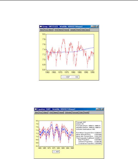
We estimate a regression of HS on a constant, SP, and the lag of HS, with an AR(1) to correct for residual serial correlation, using data for the period 1959M01–1990M12, and then use the model to forecast housing starts under a variety of settings. Following estimation, the equation results are held in the equation object EQ01:
Dependent Variable: HS
Method: Least Squares
Date: 01/15/04 Time: 15:57
Sample (adjusted): 1959M03 1990M:01
Included observations: 371 after adjusting endpoints
Convergence achieved after 4 iterations
Variable |
Coefficient |
Std. Error |
t-Statistic |
Prob. |
|
|
|
|
|
|
|
|
|
|
C |
0.321924 |
0.117278 |
2.744975 |
0.0063 |
HS(-1) |
0.952653 |
0.016218 |
58.74157 |
0.0000 |
SP |
0.005222 |
0.007588 |
0.688249 |
0.4917 |
AR(1) |
-0.271254 |
0.052114 |
-5.205027 |
0.0000 |
|
|
|
|
|
|
|
|
|
|
R-squared |
0.861373 |
Mean dependent var |
7.324051 |
|
Adjusted R-squared |
0.860240 |
S.D. dependent var |
0.220996 |
|
S.E. of regression |
0.082618 |
Akaike info criterion |
-2.138453 |
|
Sum squared resid |
2.505050 |
Schwarz criterion |
-2.096230 |
|
Log likelihood |
400.6830 |
F-statistic |
|
760.1338 |
Durbin-Watson stat |
2.013460 |
Prob(F-statistic) |
0.000000 |
|
|
|
|
|
|
|
|
|
|
|
Inverted AR Roots |
-.27 |
|
|
|
|
|
|
|
|
|
|
|
|
|
544—Chapter 18. Forecasting from an Equation
Note that the estimation sample is adjusted by two observations to account for the first difference of the lagged endogenous variable used in deriving AR(1) estimates for this model.
To get a feel for the fit of the model, select View/Actual, Fitted, Residual…, then choose
Actual, Fitted, Residual Graph:
The actual and fitted values depicted on the upper portion of the graph are virtually indistinguishable. This view provides little control over the process of producing fitted values, and does not allow you to save your fitted values. These limitations are overcome by using EViews built-in forecasting procedures to compute fitted values for the dependent variable.
How to Perform a Forecast
To forecast HS from this equation, push the Forecast button on the equation toolbar, or select Proc/Forecast….
At the top of the Forecast dialog, EViews displays information about the forecast. Here, we show a basic version of the dialog showing that we are forecasting values for the dependent series HS using the estimated EQ01. More complex settings are described in “Forecasting from Equations with Expressions” on page 561.
You should provide the following information:
Forecasting from Equations in EViews—545
•Forecast name. Fill in the edit box with the series name to be given to your forecast. EViews suggests a name, but you can change it to any valid series name. The name should be different from the name of the dependent variable, since the forecast procedure will overwrite data in the specified series.
•S.E. (optional). If desired, you may provide a name for the series to be filled with the forecast standard errors. If you do not provide a name, no forecast errors will be saved.
•GARCH (optional). For models estimated by ARCH, you will be given a further option of saving forecasts of the conditional variances (GARCH terms). See Chapter 20, “ARCH and GARCH Estimation”, on page 601 for a discussion of GARCH estimation.
•Forecasting method. You have a choice between Dynamic and Static forecast methods. Dynamic calculates dynamic, multi-step forecasts starting from the first period in the forecast sample. In dynamic forecasting, previously forecasted values for the lagged dependent variables are used in forming forecasts of the current value (see “Forecasts with Lagged Dependent Variables” on page 555 and “Forecasting with ARMA Errors” on page 557). This choice will only be available when the estimated equation contains dynamic components, e.g., lagged dependent variables or ARMA terms. Static calculates a sequence of one-step ahead forecasts, using the actual, rather than forecasted values for lagged dependent variables, if available.
You may elect to always ignore coefficient uncertainty in computing forecast standard errors (when relevant) by unselecting the Coef uncertainty in S.E. calc box.
In addition, in specifications that contain ARMA terms, you can set the Structural option, instructing EViews to ignore any ARMA terms in the equation when forecasting. By default, when your equation has ARMA terms, both dynamic and static solution methods form forecasts of the residuals. If you select Structural, all forecasts will ignore the forecasted residuals and will form predictions using only the structural part of the ARMA specification.
•Sample range. You must specify the sample to be used for the forecast. By default, EViews sets this sample to be the workfile sample. By specifying a sample outside the sample used in estimating your equation (the estimation sample), you can instruct EViews to produce out-of-sample forecasts.
Note that you are responsible for supplying the values for the independent variables in the out-of-sample forecasting period. For static forecasts, you must also supply the values for any lagged dependent variables.
•Output. You can choose to see the forecast output as a graph or a numerical forecast evaluation, or both. Forecast evaluation is only available if the forecast sample includes observations for which the dependent variable is observed.
546—Chapter 18. Forecasting from an Equation
•Insert actuals for out-of-sample observations. By default, EViews will fill the forecast series with the values of the actual dependent variable for observations not in the forecast sample. This feature is convenient if you wish to show the divergence of the forecast from the actual values; for observations prior to the beginning of the forecast sample, the two series will contain the same values, then they will diverge as the forecast differs from the actuals. In some contexts, however, you may wish to have forecasted values only for the observations in the forecast sample. If you uncheck this option, EViews will fill the out-of-sample observations with missing values.
Note that when performing forecasts from equations specified using expressions or autoupdating series, you may encounter a version of the Forecast dialog that differs from the basic dialog depicted above. See “Forecasting from Equations with Expressions” on page 561 for details.
An Illustration
Suppose we produce a dynamic forecast using EQ01 over the sample 1959M01 to 1996M01. The forecast values will be placed in the series HSF, and EViews will display both a graph of the forecasts and the plus and minus two standard error bands, as well as a forecast evaluation:
This is a dynamic forecast for the period from 1989M01 through 1996M01. For every period, the previously forecasted values for HS(-1) are used in forming a forecast of the subsequent value of HS. As noted in the output, the forecast values are saved in the series HSF. Since HSF is a standard EViews series, you may examine your forecasts using all of the standard tools for working with series objects.
An Illustration—547
For example, we may examine the actual versus fitted values by creating a group containing HS and HSF, and plotting the two series. Click on Quick/Show… and enter “HS” and “HSF”. Then select View/Graph/Line to display the two series:
Note the considerable difference between this actual and fitted graph and the Actual, Fitted, Residual Graph depicted above.
To perform a series of one-step ahead forecasts, click on Forecast on the equation toolbar, and select Static forecasts. EViews will display the forecast results:
We may also compare the actual and fitted values from the static forecast by examining a line graph of a group containing HS and the new HSF.
548—Chapter 18. Forecasting from an Equation
The one-step ahead static forecasts are more accurate than the dynamic forecasts since, for each period, the actual value of HS(-1) is used in forming the forecast of HS. These onestep ahead static forecasts are the same forecasts used in the Actual, Fitted, Residual Graph displayed above.
Lastly, we construct a dynamic forecast beginning in 1990M02 (the first period following the estimation sample) and ending in 1996M01. Keep in mind that data are available for SP for this entire period. The plot of the actual and the forecast values for 1989M01 to 1996M01 is given by:
Since we use the default settings for out-of-forecast sample values, EViews backfills the forecast series prior to the forecast sample (up through 1990M01), then dynamically forecasts HS for each subsequent period through 1996M01. This is the forecast that you would