838—Chapter 27. Pooled Time Series, Cross-Section Data
Working with Pooled Data
The underlying series for each cross-section member are ordinary series, so all of the EViews tools for working with the individual cross-section series are available. In addition, EViews provides you with a number of specialized tools which allow you to work with your pool data. Using EViews, you can perform, in a single step, similar operations on all the series corresponding to a particular pooled variable.
Generating Pooled Data
You can generate or modify pool series using the pool series genr procedure. Click on PoolGenr on the pool toolbar and enter a formula as you would for a regular genr, using pool series names as appropriate. Using our example from above, entering:
ratio? = g?/g_usa
is equivalent to entering the following four commands:
ratio_usa = g_usa/g_usa
ratio_uk = g_uk/g_usa
ratio_jpn = g_jpn/g_usa
ratio_kor = g_kor/g_usa
Generation of a pool series applies the formula you supply using an implicit loop across cross-section identifiers, creating or modifying one or more series as appropriate.
You may use pool and ordinary genr together to generate new pool variables. For example, to create a dummy variable that is equal to 1 for the US and 0 for all other countries, first select PoolGenr and enter:
dum? = 0
to initialize all four of the dummy variable series to 0. Then, to set the US values to 1, select Quick/Generate Series… from the main menu, and enter:
dum_usa = 1
It is worth pointing out that a superior method of creating this pool series is to use @GROUP to define a group called US containing only the “_USA” identifier (see “Group Definitions” on page 828), then to use the @INGRP function:
dum? = @ingrp(us)
to generate and implicitly refer to the four series (see “Pool Series” on page 830).
To modify a set of series using a pool, select PoolGenr, and enter the new pool series expression:
Working with Pooled Data—839
dum? = dum? * (g? > c?)
It is worth the reminder that the method used by the pool genr is to perform an implicit loop across the cross-section identifiers. This implicit loop may be exploited in various ways, for example, to perform calculations across cross-sectional units in a given period. Suppose, we have an ordinary series SUM which is initialized to zero. The pool genr expression:
sum = sum + c?
is equivalent to the following four ordinary genr statements:
sum = sum + c_usa sum = sum + c_uk sum = sum + c_jpn sum = sum + c_kor
Bear in mind that this example is provided merely to illustrate the notion of implicit looping, since EViews provides built-in features to compute period-specific statistics.
Examining Your Data
Pool workfiles provide you with the flexibility to examine cross-section specific series as individual time series or as part of a larger set of series.
Examining Unstacked Data
Simply open an individual series and work with it using the standard tools available for examining a series object. Or create a group of series and work with the tools for a group object. One convenient way to create groups of series is to use tools for creating groups out of pool and ordinary series; another is to use wildcards expressions in forming the group.
Examining Stacked Data
As demonstrated in “Stacked Data” beginning on page 833, you may use your pool object to view your data in stacked spreadsheet form. Select View/Spreadsheet View…, and list the series you wish to display. The names can include both ordinary and pool series names. Click on the Order +/– button to toggle between stacking your observations by cross-section and by date.
We emphasize that stacking your data only provides an alternative view of the data, and does not change the structure of the individual series in your workfile. Stacking data is not necessary for any of the data management or estimation procedures described below.
840—Chapter 27. Pooled Time Series, Cross-Section Data
Calculating Descriptive Statistics
EViews provides convenient built-in features for computing various descriptive statistics for pool series using a pool object. To display the Pool Descriptive Statistics dialog, select
View/Descriptive Statistics… from the pool toolbar.
In the edit box, you should list the ordinary and pooled series for which you want to compute the descriptive statistics. EViews will compute the mean, median, minimum, maximum, standard deviation, skewness, kurtosis, and the Jarque-Bera statistic for these series.
First, you should choose between the three sample options on the right of the dialog:
•Individual: uses the maximum number of observations available. If an observation on a variable is available for a particular crosssection, it is used in computation.
•Common: uses an observation only if data on the variable are available for all crosssections in the same period. This method is equivalent to performing listwise exclusion by variable, then cross-sectional casewise exclusion within each variable.
•Balanced: includes observations when data on all variables in the list are available for all cross-sections in the same period. The balanced option performs casewise exclusion by both variable and cross-section.
Next, you should choose the computational method corresponding to one of the four data structures:
•Stacked data: display statistics for each variable in the list, computed over all crosssections and periods. These are the descriptive statistics that you would get if you ignored the pooled nature of the data, stacked the data, and computed descriptive statistics.
•Stacked – means removed: compute statistics for each variable in the list after removing the cross-sectional means, taken over all cross-sections and periods.
•Cross-section specific: show the descriptive statistics for each cross-sectional variable, computed across all periods. These are the descriptive statistics derived by computing statistics for the individual series.
•Time period specific: compute period-specific statistics. For each period, compute the statistic using data on the variable from all the cross-sectional units in the pool.
Working with Pooled Data—841
Click on OK, and EViews will display a pool view containing tabular output with the requested statistics. If you select Stacked data or Stacked - means removed, the view will show a single column containing the descriptive statistics for each ordinary and pool series in the list, computed from the stacked data. If you select Cross-section specific, EViews will show a single column for each ordinary series, and multiple columns for each pool series. If you select Time period specific, the view will show a single column for each ordinary or pool series statistic, with each row of the column corresponding to a period in the workfile. Note that there will be a separate column for each statistic computed for an ordinary or pool series; a column for the mean, a column for the variance, etc.
You should be aware that the latter two methods may produce a great deal of output. Cross-section specific computation generates a set of statistics for each pool series/crosssection combination. If you ask for statistics for three pool series and there are 20 crosssections in your pool, EViews will display 60 columns of descriptive statistics. For time period specific computation, EViews computes a set of statistics for each date/series combination. If you have a sample with 100 periods and you provide a list of three pool series, EViews will compute and display a view with columns corresponding to 3 sets of statistics, each of which contains values for 100 periods.
If you wish to compute period-specific statistics, you may alternatively elect to save the results in series objects. See “Making Period Stats” on page 842.
Computing Unit Root Tests
EViews provides convenient tools for computing multiple-series unit root tests for pooled data using a pool object. You may use the pool to compute one or more of the following types of unit root tests: Levin, Lin and Chu (2002), Breitung (2002), Im, Pesaran and Shin (2003), Fisher-type tests using ADF and PP tests—Maddala and Wu (1999) and Choi (2001), and Hadri (1999).
To compute the unit root test, select View/Unit Root Test…from the menu of a pool object.
842—Chapter 27. Pooled Time Series, Cross-Section Data
Enter the name of an ordinary or pool series in the topmost edit field, then specify the remaining settings in the dialog.
These tests, along with the settings in the dialog, are described in considerable detail in “Panel Unit Root Tests” on page 530.
Making a Group of Pool
Series
If you click on Proc/Make Group… and enter the names
of ordinary and pool series. EViews will use the pool definitions to create an untitled group object containing the specified series. This procedure is useful when you wish to work with a set of pool series using the tools provided for groups.
Suppose, for example, that you wish to compute the covariance matrix for the C? series. Simply open the Make Group dialog, and enter the pool series name C?. EViews will create a group containing the set of cross-section specific series, with names beginning with “C” and ending with a cross-section identifier.
Then, in the new group object, you may select View/Covariances and either Common Sample or Pairwise Sample to describe the handling of missing values. EViews will display a view of the covariance matrix for all of the individual series in the group. Each element represents a covariance between individual members of the set of series in the pool series C?.
Making Period Stats
To save period-specific statistics in series in the workfile, select Proc/Make Period Stat Series… from the pool window, and fill out the dialog.
Working with Pooled Data—843
In the edit window, list the series for which you wish to calculate period-statistics. Next, select the particular statistics you wish to compute, and choose a sample option.
EViews will save your statistics in new series and will open an untitled group window to display the results. The series will be named automatically using the base name followed by the name of the statistic (MEAN, MED, VAR, SD, OBS, SKEW, KURT, JARQ, MAX, MIN). In this example, EViews will save the statistics using the names CMEAN, GMEAN, CVAR, GVAR, CMAX, GMAX, CMIN, and GMIN.
Making a System
Suppose that you wish to estimate a complex specification that cannot easily be estimated using the built-in features of the pool object. For example, you may wish to estimate a pooled equation imposing arbitrary coefficient restrictions, or using specialized GMM techniques that are not available in pooled estimation.
In these circumstances, you may use the pool to create a system object using both common and cross-section specific coefficients, AR terms, and instruments. The resulting system object may then be further customized, and estimated using all of the techniques available for system estimation.
Select Proc/Make System… and fill out the dialog. You may enter the dependent variable, common and cross-section specific variables, and use the checkbox to allow for crosssectional fixed effects. You may also enter a list of common and cross-section specific instrumental variables, and instruct EViews to add lagged dependent and independent regressors as instruments in models with AR specifications.
844—Chapter 27. Pooled Time Series, Cross-Section Data
When you click on OK, EViews will take your specification and create a new system object containing a single equation for each cross-section, using the specification provided.
Deleting/Storing/Fetching Pool Data
Pools may be used to delete, store, or fetch sets of series. Simply select Proc/Delete pool series…, Proc/Store pool series (DB)…, or Proc/Fetch pool series (DB)… as appropriate, and enter the ordinary and pool series names of interest.
If, for example, you instruct EViews to delete the pool series C?, EViews will loop through all of the cross-section identifiers and delete all series whose names begin with the letter “C” and end with the cross-section identifier.
Exporting Pooled Data
You can export your data into a disk file, or into a new workfile or workfile page, by reversing one of the procedures described above for data input.
To write pooled data in stacked form into an ASCII text, Excel, or Lotus worksheet file, first open the pool object, then from the pool menu, select Proc/
Import Pool data (ASCII,
.XLS, .WK?)…. Note that in order to access the pool specific export tools, you must select this procedure from the pool menu, not from the workfile menu.
EViews will first open a file
dialog prompting you to specify a file name and type. If you provide a new name, EViews will create the file; otherwise it will prompt you to overwrite the existing file.
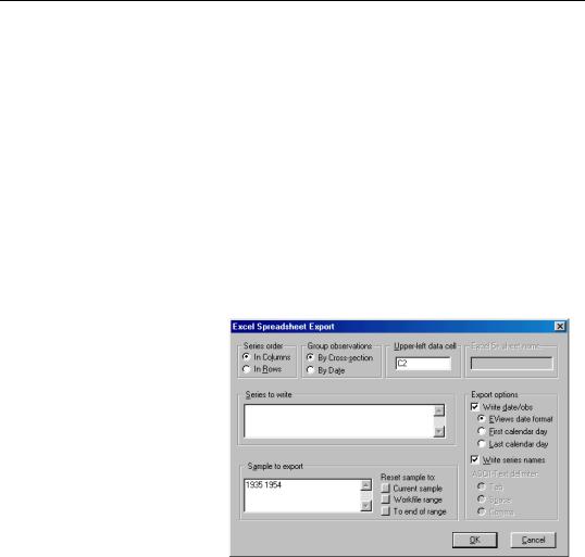
Once you have specified your file, a pool write dialog will be displayed. Here we see the Excel Spreadsheet Export dialog. Specify the format of your data, including whether to write series in columns or in rows, and whether to stack by cross-section or by period.
Then list the ordinary series, groups, and pool series to be written to the file, the sample of observations to be written, and select any export options. When you click on OK, EViews will write the specified file.