


Reshaping a Workfile—241
tions for type; an object will be copied only if it is in the list of object names provided in the edit box, and if its type matches a classification that you elect to copy. If, for example, you wish to remove all objects that are not series objects or valmaps from your list, you should uncheck the Estimation & Model objects and the All others checkboxes.
Lastly, you may optionally provide a destination workfile page. By default, EViews will copy the data to a new workfile in a page named after the workfile page structure (e.g., “Quarterly”, “Monthly”). You may provide an alternative destination by clicking on the Page Destination tab in the dialog, and entering the desired destination workfile and/or page.
When you click on OK, EViews examines your source workfile and the specified sample, and creates a new page with the appropriate number of observations. EViews then copies the ID series used to structure the source workfile, and structures the new workfile in identical fashion. Lastly, the specified objects are copied to the new workfile page.
Reshaping a Workfile
In a typical study, each subject (individual, firm, period, etc.) is observed only once. In these cases, each observation corresponds to a different subject, and each series, alpha, or link in the workfile represents a distinct variable.
In contrast, repeated measures data may arise when the same subject is observed at different times or under different settings. The term repeated measures comes from the fact that for a given subject we may have repeated values, or measures, for some variables. For example, in longitudinal surveys, subjects may be asked about their economic status on an annual basis over a period of several years. Similarly, in clinical drug trials, individual patient health may be observed after several treatment events.
It is worth noting that standard time series data may be viewed as a special case of repeated measures data, in which there are repeated higher frequency observations for each lower frequency observation. Quarterly data may, for example, be viewed as data in which there are four repeated values for each annual observation. While time series data are not typically viewed in this context, the interpretation suggests that the reshaping tools described in this section are generally applicable to time series data.
There are two basic ways that repeated measures data may be organized in an EViews workfile. To illustrate the different formats, we consider a couple of simple examples.
Suppose that we have the following dataset:

242—Chapter 9. Advanced Workfiles
ID1 |
ID2 |
Sales |
|
|
|
1 |
Jason |
17 |
|
|
|
1 |
Adam |
8 |
|
|
|
2 |
Jason |
30 |
|
|
|
2 |
Adam |
12 |
|
|
|
3 |
Jason |
20 |
|
|
|
We may view these data as representing repeated measures on subjects with identifiers given in ID1, or as repeated measures for subjects with names provided in ID2. There are, for example, two repeated values for subjects with “ID1=1”, and three repeated values for SALES for Jason. Note that in either case, the repeated values for the single series SALES are represented in multiple observations.
We can rearrange the layout of the data into an equivalent form where the values of ID2 are used to break SALES into multiple series (one for each distinct value of ID2):
ID1 |
SalesJason |
SalesAdam |
|
|
|
1 |
17 |
8 |
|
|
|
2 |
30 |
12 |
|
|
|
3 |
20 |
NA |
|
|
|
The series ID2 no longer exists as a distinct series in the new format, but instead appears implicitly in the names associated with the new series (SALESJASON and SALESADAM). The repeated values for SALES are no longer represented by multiple observations, but are instead represented in the multiple series values associated with each value of ID1.
Note also that this representation of the data requires that we add an additional observation corresponding to the case ID1=3, ID2=“Adam”. Since the observation did not exist in the original representation, the corresponding value of SALESADAM is set to NA.
Alternatively, we may rearrange the data using the values in ID1 to break SALES into multiple series:
ID2 |
Sales1 |
Sales2 |
Sales3 |
|
|
|
|
Jason |
17 |
30 |
20 |
|
|
|
|
Adam |
8 |
12 |
NA |
|
|
|
|
In this format, the series ID1 no longer exists as a distinct series, but appears implicitly in the series names for SALES1, SALES2, and SALES3. Once again, the repeated responses for

Reshaping a Workfile—243
SALES are not represented by multiple observations, but are instead held in multiple series.
The original data format is often referred to as repeated observations format, since multiple observations are used to represent the SALES data for an individual ID1 or ID2 value. The latter two representations are said to be in repeated variable or multivariate form since they employ multiple series to represent the SALES data.
When data are rearranged so that a single series in the original workfile is broken into multiple series in a new workfile, we term the operation unstacking the workfile. Unstacking a workfile converts data from repeated observations to multivariate format.
When data are rearranged so that sets of two or more series in the original workfile are combined to form a single series in a new workfile, we call the operation stacking the workfile. Stacking a workfile converts data from multivariate to repeated observations format.
In a time series context, we may have the data in the standard stacked format:
Date |
Year |
Quarter |
Z |
|
|
|
|
2000Q1 |
2000 |
1 |
2.1 |
|
|
|
|
2000Q2 |
2000 |
2 |
3.2 |
|
|
|
|
2000Q3 |
2000 |
3 |
5.7 |
|
|
|
|
2000Q4 |
2000 |
4 |
6.3 |
|
|
|
|
2001Q1 |
2001 |
1 |
7.4 |
|
|
|
|
2001Q2 |
2001 |
2 |
8.1 |
|
|
|
|
2001Q3 |
2001 |
3 |
8.8 |
|
|
|
|
2001Q4 |
2001 |
4 |
9.2 |
|
|
|
|
where we have added the columns labeled YEAR and QUARTER so that you may more readily see the repeated measures interpretation of the data.
We may rearrange the time series data so that it is unstacked by QUARTER,
Year |
Z1 |
Z2 |
Z3 |
Z4 |
|
|
|
|
|
2000 |
2.1 |
3.2 |
5.7 |
6.3 |
|
|
|
|
|
2001 |
7.4 |
8.1 |
8.8 |
9.2 |
|
|
|
|
|
or in the alternative form where it is unstacked by YEAR:

244—Chapter 9. Advanced Workfiles
Quarter |
Z2000 |
Z2001 |
|
|
|
1 |
2.1 |
7.4 |
|
|
|
2 |
3.2 |
8.1 |
|
|
|
3 |
5.7 |
8.8 |
|
|
|
4 |
6.2 |
9.2 |
|
|
|
EViews provides you with convenient tools for reshaping workfiles between these different formats. These tools make it easy to prepare a workfile page that is set up for use with built-in pool or panel data features, or to convert data held in one time series representation into an alternative format.
Unstacking a Workfile
Unstacking a workfile involves taking series objects in a workfile page, and in a new workfile, breaking the original series into multiple series.
We employ an unstacking ID series in the original workfile to determine the destination series, and an observation ID series to determine the destination observation, for every observation in the original workfile. Accordingly, we say that a workfile is “unstacked by” the values of the unstacking ID series.
To ensure that each series observation in the new workfile contains no more than one observation from the existing workfile, we require that the unstacking ID and the observation ID are chosen such that no two observations in the original workfile have the same set of values for the identifier series. In other words, the identifier series must together uniquely identify observations in the original workfile.
While you may use any series in the workfile as your unstacking and observation identifier series, an obvious choice for the identifiers will come from the set of series used to structure the workfile (if available). In a dated panel, for example, the cross-section ID and date ID series uniquely identify the rows of the workfile. We may then choose either of these series as the unstacking ID, and the other as the observation ID.
If we unstack the data by the cross-section ID, we end up with a simple dated workfile with each existing series split into separate series, each corresponding to a distinct crosssection ID value. This is the workfile structure used by the EViews pool object, and is commonly used when the number of cross-sectional units is small. Accordingly, one important application of unstacking a workfile involves taking a page with a panel structure and creating a new page suitable for use with EViews pool objects.
On the other hand, if we unstack the panel workfile by date (using the date ID series or @DATE), we end up with a workfile where each row represents a cross-sectional unit, and

Reshaping a Workfile—245
each original series is split into separate series, one for each observed time period. This format is frequently used in the traditional repeated measures setting where a small number of variables in a cross-sectional dataset have been observed at different times.
To this point, we have described the unstacking of panel data. Even if your workfile is structured using a single identifier series, however, it may be possible to unstack the workfile by first splitting the single identifier into two parts, and using the two parts as the identifier series. For example, consider the simple quarterly data given by:
Date |
X |
Y |
|
|
|
2000Q1 |
NA |
-2.3 |
|
|
|
2000Q2 |
5.6 |
-2.3 |
|
|
|
2000Q3 |
8.7 |
-2.3 |
|
|
|
2000Q4 |
9.6 |
-2.3 |
|
|
|
2001Q1 |
12.1 |
1.6 |
|
|
|
2001Q2 |
8.6 |
1.6 |
|
|
|
2001Q3 |
14.1 |
1.6 |
|
|
|
2001Q4 |
15.2 |
1.6 |
|
|
|
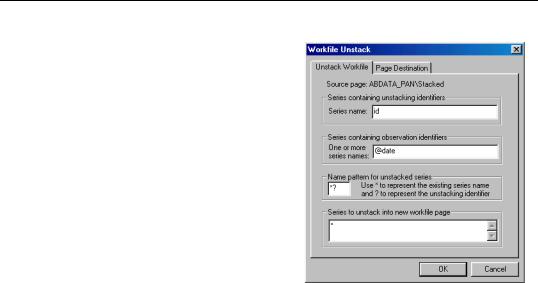
Suppose we wish to unstack the X series. We may split the date identifier into a year component and a quarter component (using, say, the EViews @YEAR and @QUARTER functions). If we extract the QUARTER and YEAR from the date and use the QUARTER as the unstacking identifier, and the YEAR as the observation identifier, we obtain the unstacked data:
Year |
X1 |
X2 |
X3 |
X4 |
|
|
|
|
|
2000 |
NA |
5.6 |
8.7 |
9.6 |
|
|
|
|
|
2001 |
12.1 |
8.6 |
14.1 |
15.2 |
|
|
|
|
|
Note that we have chosen to form the series names by concatenating the name of the X series, and the values of the QUARTER series.
Alternatively, if we use YEAR as the unstacking ID, and QUARTER as the observation ID, we have:

246—Chapter 9. Advanced Workfiles
Quarter |
X2000 |
X2001 |
|
|
|
1 |
NA |
12.1 |
|
|
|
2 |
5.6 |
8.6 |
|
|
|
3 |
8.7 |
14.1 |
|
|
|
4 |
9.6 |
15.2 |
|
|
|
In some cases, a series in the original workfile will not vary by the unstacking ID. In our example, we have a series Y that is only updated once a year. Stacking by QUARTER yields:
Year |
Y1 |
Y2 |
Y3 |
Y4 |
|
|
|
|
|
2000 |
-2.3 |
-2.3 |
-2.3 |
-2.3 |
|
|
|
|
|
2001 |
1.6 |
1.6 |
1.6 |
1.6 |
|
|
|
|
|
Since there is no change in the observations across quarters, these data may be written as:
Year |
Y |
|
|
2000 |
-2.3 |
|
|
2001 |
1.6 |
|
|
without loss of information. When unstacking, EViews will automatically avoid splitting any series which does not vary across different values of the unstacking ID. Thus, if you ask EViews to unstack the original Y by QUARTER, only the compacted (single series) form will be saved. Note that unstacking by YEAR will not produce a compacted format since Y is not constant across values of YEAR for a given value of QUARTER.
Unstacking a Workfile in EViews
To unstack the active workfile page, you should select Proc/Reshape Current Page/ Unstack in New Page... from the main workfile menu. EViews will respond by opening the tabbed Workfile Unstack dialog.
Reshaping a Workfile—247
When unstacking data, there are four key pieces of information that should be provided: a series object that contains the unstacking IDs, a series object that contains the observation IDs, the series in the source workfile that you wish to unstack, and a rule for defining names for the unstacked series.
Unstacking Identifiers
To unstack data contained in a workfile page, your source page must contain a series object containing the unstacking identifiers associated with each observation. For example, you may have an alpha series containing country abbreviations (“US”, “JPN”, “UK”), or individual names (“Joe Smith”, “Jane Doe”), or a
numeric series with integer identifiers (“1”, “2”, “3”, “50”, “100”, ...). Typically, there will be repeated observations for each of the unique unstacking ID values.
You should provide the name of your unstacking ID series object in the top edit field of the dialog. When unstacking, EViews will create a separate series for each distinct value of the ID series, with each of these series containing the multiple observations associated with that value. The series used as the unstacking ID is always dropped from the destination workfile since its values are redundant since they are built into the multiple series names.
If you wish to unstack using values in more than one series, you must create a new series that combines the two identifiers by identifying the subgroups, or you may simply repeat the unstacking operation.
Observation Identifiers
Next, you must specify a series object containing an observation ID series in the second edit field. The values of this series are used to identify both the individual observations in the unstacked series and the structure of the destination page.
Once again, if your workfile is structured, an obvious choice for the unstacking identifier series comes from the series used to structure the workfile, either directly (the date or cross-section ID in a panel page), or indirectly (the YEAR or QUARTER extracted from a quarterly date).
EViews will, if necessary, create a new observation ID series in the unstacked page with the same name as, and containing the unique values of, the original observation ID series. This series will be used to structure the workfile.

248—Chapter 9. Advanced Workfiles
If the original observation ID is an ordinary series or alpha, the new page will be structured as a cross-section page using the new identifier series. Alternatively, if the observation ID is a date series or the “@DATE” keyword, EViews will analyze the observed date values and will create a dated page with the appropriate frequency.
Series to be Unstacked
You may enter the names of the series, alphas, and links that you wish to unstack in the edit field Series to be unstacked into new workfile page. You may enter the names directly, or use expressions containing wildcards. For example, the expression “SALES A*” instructs EViews to unstack both the SALES series as well as all series objects beginning with the letter “A”.
Note that the RESID series and the unstacking ID series may not be unstacked.
Naming Unstacked Series
EViews will use the pattern in the Name pattern for unstacked series field to construct the names for the new unstacked series or alphas associated with each stacked series object.
By default, the wildcard pattern “*?” will be used, meaning that unstacked series names will be constructed by concatenating the name of the series object to be unstacked and a string containing one of the unique values found in the unstacking ID series.
In our example above, when unstacking the SALES series using NAME as the unstacking ID series and the wildcard name pattern “*?”, EViews will create the series JASONSALES and ADAMSALES. If instead, we enter the pattern “?_*”, EViews will put the unstacked values in the series SALES_JASON and SALES_ADAM.
Unstacking Destination
By default, EViews will unstack the data in a new UNTITLED page in the existing workfile. You may provide an alternative destination by clicking on the Page Destination tab in the dialog, and entering the desired destination.
Reshaping a Workfile—249
An Example
Consider a workfile that contains the series GDP and CONS, which contain the values of Gross Domestic Product and consumption for three countries stacked on top of each other.
Suppose further that there is an alpha object called COUNTRY containing the values “US”, “UK”, and “JPN”, which identify the country associated with each observation on GDP and CONS. Finally, suppose there is a date series DATEID
which identifies the date associated with each observation in the page. COUNTRY and DATEID uniquely determine the observation identifiers.
In our example, we assume that the source page contains annual data from 1991 to 2000 for the three countries in our panel. We can better see this structure by opening a group window showing the values of COUNTRY, DATEID (displayed in year-date format), and GDP.
We wish to unstack the data in GDP and CONS using the unstacking ID values in COUN-
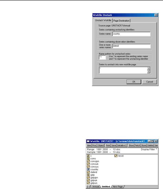
TRY, and the observation IDs in DATEID. Click on Proc/Reshape Current Page/Unstack in New Page... in the workfile window to bring up the unstacking dialog.
250—Chapter 9. Advanced Workfiles
Enter “COUNTRY” as the unstacking ID series, and “DATEID” for the observation identifier. We leave the remainder of the dialog settings at the default values, so that EViews will use “*?” as the name pattern, will copy all series objects in the page (with the exception of RESID and COUNTRY), and will place the results in a new page in the same workfile.
If you click on OK to accept the settings, EViews will first examine the DATEID series to determine the number of unique observation identifiers. Note that the number of unique observation identifier values determines the number of observations in the
unstacked workfile. Next, EViews will determine the number of unique values in COUNTRY, which is equal to the number of unstacked series created for each stacked series.
In this example, we start with a balanced panel with 10 distinct values for DATEID, and three distinct values in COUNTRY. The resulting UNTITLED workfile page will follow an annual frequency from the 10 observations from 1991 to 2000, and will have three unstacked series corresponding to each of the source series. The names of these series will be formed by taking the original series name and appending the distinct values in COUNTRY (“US”, “UK”, and “JPN”).
Note that in addition to the six unstacked series CONSJPN, CONSUK, CONSUS, GDPJPN, GDPUK, GDPUS, EViews has created four additional objects. First, the unstacked page contains two group objects taking the name of, and corresponding to, the original series CONS and GDP.
Each group contains all of the unstacked series, providing you with easy access to all of the series associated with the origi-
nal stacked series. For example, the group GDP contains the three series, GDPJPN, GDPUK, and GDPUS, while CONS contains CONSJPN, CONSUK, and CONSUS.

Reshaping a Workfile—251
Opening the GDP group spreadsheet, we see the result of unstacking the original GDP series into three series: GDPJPN, GDPUK, and GDPUS. In particular, the values of the GDPJPN and GDPUK series should be compared with the values of GDP depicted in the group spreadsheet view of the stacked data.
Second, EViews has created a (date) series DATEID containing the distinct values of the observation ID series. If
necessary, this series will be used to structure the unstacked workfile.
Lastly, EViews has created a pool object named COUNTRY, corresponding to the specified unstack ID series, containing all of the unstacking identifiers. Since the unstacked series have names that were created using the specified name pattern, this pool object is perfectly set up for working with the unstacked data.
Stacking a Workfile
Stacking a workfile involves combining sets of series with related names into single series, or repeatedly stacking individual series into single series, and placing the results in a new workfile. The series in a given set to be stacked may be thought of as containing repeated measures data on a given variable. The individual series may be viewed as ordinary, nonrepeated measures data.
The stacking operation depends crucially on the set of stacking identifiers. These identifiers are used to determine the sets of series, and the number of times to repeat the values of individual series.
In order for all of the series in a given set to be stacked, they must have names that contain a common component, or base name, and the names must differ systematically in containing an identifier. The identifiers can appear as a suffix, prefix, or even in the middle of the base name, but they must be used consistently across all series in each set.
Suppose, for example, we have a workfile containing the individual series Z, and the two groups of series: XUS, XUK and XJPN, and US_Y, UK_Y, and JPN_Y. Note that within each set of series, the identifiers “US”, “UK”, and “JPN” are used, and that they are used consistently within each set of series.
If we employ the set of three identifier values “US”, “UK”, and “JPN” to stack our workfile, EViews will stack the three series XUS, XUK, and XJPN on top of each other, and the series US_Y, UK_Y, and JPN_Y on top of each other. Furthermore, the individual series Z will be

252—Chapter 9. Advanced Workfiles
stacked on top of itself three times so that there are three copies of the original data in the new series.
Stacking a Workfile in EViews
To stack the data in an existing workfile page, you should select Proc/Reshape Current Page/Stack in New Page... from the main workfile menu. EViews will respond by opening the tabbed Workfile Stack dialog.
There are two key pieces of information that you must provide in order to create a stacked workfile: the set of stack ID values, and the series that you wish to stack. This information should be provided in the two large edit fields. The remaining dialog settings involve options that allow you to modify the method used to stack the series and the destination of the stacked series.
Stacking Identifiers
There are three distinct methods that you may use to specify your stack ID values:
First, you may enter a space separated
list containing the individual ID values (e.g., “1 2 3”, or “US UK JPN”). This is the most straightforward method, but can be cumbersome if you have a large list of values.
Second, you may enter the name of an existing pool object that contains the identifier values.
Lastly, you may instruct EViews to extract the ID values from a set of series representing repeated measures on some variable. To use this method, you should enter a series name pattern containing the base name and the “?” character in place of the IDs. EViews will use this expression to identify a set of series, and will extract the ID values from the series names. For example, if you enter “SALES?”, EViews will identify all series in the workfile with names beginning with the string “SALES”, and will form a list of identifiers from the remainder of the observed series names. In our example, we have the series SALES1, SALES2, and SALES3 in the workfile, so that the list of IDs will be “1”, “2”, and “3”.
Series to be Stacked
Next, you should enter the list of series, alphas, and links that you wish to stack. Sets of series objects that are to be treated as repeated measures (stacked on top of each other)

Reshaping a Workfile—253
should be entered using “?” series name patterns, while individual series (those that should be repeatedly stacked on top of themselves), should be entered using simple names or wildcards.
You may specify the repeated measures series by listing individual stacked series with “?” patterns (“CONS? EARN?”), or you may use expressions containing the wildcard character “*” (“*?” and “?C*”) to specify multiple sets of series. For example, entering the expression “?C* ?E*” will tell EViews to find all repeated measures series that begin with the letters “C” or “E” (e.g., “CONS? CAP? EARN? EXPER?”), and then to stack (or interleave) the series using the list of stack ID values. If one of the series associated with a particular stack ID does not exist, the corresponding stacked values will be assigned the value NA.
Individual series may also be stacked. You may list the names of individual simple series (e.g., “POP INC”), or you can specify your series using expressions containing the wildcard character “*” (“*”, “*C”, “F*”). The individual series will repeatedly be stacked (or interleaved), once for each ID value. If the target workfile page is in the same workfile, EViews will create a link in the new page; otherwise, the stacked series will contain repeated copies of the original values.
It should be noted that the wildcard values for individual series are processed after the repeated measures series are evaluated, so that a given series will only be used once. If a series is used as part of a repeated measures series, it will not be used when matching wildcards in the list of individual series to be stacked.
The default value “*? *” is suitable for settings where the repeated series have names formed by taking the base name and appending the stack ID values. The default will stack all repeated measures series, and all remaining individual series (except for RESID). Entering “*” alone will copy or link all series, but does not identify any repeated measures series.
Naming Stacked Series
Stacked individual series will be named in the destination page using the name of the series in the original workfile; stacked repeated measures series will, by default, be named using the base name. For example, if you stack the repeated measures series “SALES?” and the individual series GENDER, the corresponding stacked series will, by default, be named “SALES” and “GENDER”, respectively.
This default rule will create naming problems when the base name of a repeated measures series is also the name of an individual series. Accordingly, EViews allows you to specify an alternative rule for naming your stacked repeated measures series in the Name for stacked series section of the dialog.
The default naming rule may be viewed as one in which we form names by replacing the “?” in the original specification with a blank space. To replace the “?” with a different

254—Chapter 9. Advanced Workfiles
string, you should enter the desired string in the edit field. For example, if you enter the string “_STK”, then EViews will name the stacked series “CONS?” and “EARN?” as “CONS_STK” and “EARN_STK” in the destination workfile.
Stacking Order
EViews will, by default, create series in the new page by stacking series on top of one another. If we have identifiers “1”, “2”, and “3”, and the series SALES1, SALES2, and SALES3, EViews will stack the entire series SALES1 followed by the entire series SALES2, followed by SALES3.
You may instruct EViews to interleave the data, by selecting the Interleaved radio button in the Order of Obs section of the dialog. If selected, EViews will stack the first observations for SALES1, SALES2, and SALES3, on top of the second observations, and so forth.
It is worth pointing out that stacking by series means that the observations contained in a given series will be kept together in the stacked form, while interleaving the data implies that the multiple values for a given original observation will be kept together. In some contexts, one form may be more natural than another.
In the case where we have time series data with different series representing different countries, stacking the data by series means that we have the complete time series for the “US” (USGDP), followed by the time series for the “UK” (UKGDP), and then “JPN” (JPNGDP). This representation is more natural for time series analysis than interleaving so that the observations for the first year are followed by the observations for the second year, and so forth.
Alternatively, where the series represent repeated measures for a given subject, stacking the data by series arranges the data so that all of the first measures are followed by all of the second measures, and so on. In this case, it may be more natural to interleave the data, so that all of the observations for the first individual are followed by all of the observations for the second individual, and so forth.
One interesting case where interleaving may be desirable is when we have data which has been split by period, within the year. For example, we may have four quarters of data for each year:
Year |
XQ1 |
XQ2 |
XQ3 |
XQ4 |
|
|
|
|
|
2000 |
NA |
5.6 |
8.7 |
9.6 |
|
|
|
|
|
2001 |
12.1 |
8.6 |
14.1 |
15.2 |
|
|
|
|
|
If we stack the series using the identifier list “Q1 Q2 Q3 Q4”, we get the data:

Reshaping a Workfile—255
Year |
ID01 |
X |
|
|
|
2000 |
Q1 |
NA |
|
|
|
2001 |
Q1 |
12.1 |
|
|
|
2000 |
Q2 |
5.6 |
|
|
|
2001 |
Q2 |
8.6 |
|
|
|
2000 |
Q3 |
8.7 |
|
|
|
2001 |
Q3 |
14.1 |
|
|
|
2000 |
Q4 |
9.6 |
|
|
|
2001 |
Q4 |
15.2 |
|
|
|
which is not ordered in the traditional time series format from earliest to latest. If instead, we stack by “Q1 Q2 Q3 Q4” but interleave, we obtain the standard format:
Year |
ID01 |
X |
|
|
|
2000 |
Q1 |
NA |
|
|
|
2000 |
Q2 |
5.6 |
|
|
|
2000 |
Q3 |
8.7 |
|
|
|
2000 |
Q4 |
9.6 |
|
|
|
2001 |
Q1 |
12.1 |
|
|
|
2001 |
Q2 |
8.6 |
|
|
|
2001 |
Q3 |
14.1 |
|
|
|
2001 |
Q4 |
15.2 |
|
|
|
Note that since interleaving changes only the order of the observations in the workfile and not the structure, we can always sort or restructure the workfile at a later date to achieve the same effect.
Stacking Destination
By default, EViews will stack the data in a new page in the existing workfile named “UNTITLED” (or the next available name, “UNTITLED1”, “UNTITLED2”, etc., if there are existing pages in the workfile with the same name).
256—Chapter 9. Advanced Workfiles
You may provide an alternative destination for the stacked data by clicking on the Page Destination tab in the dialog, and entering the desired destination.
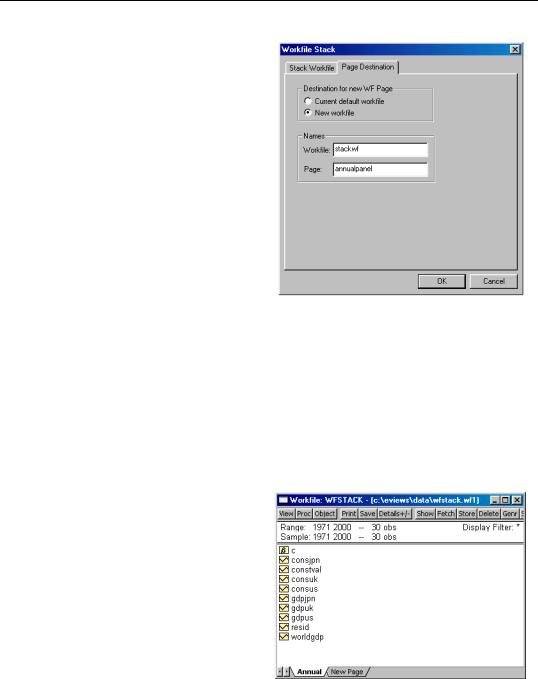
Here, we instruct EViews to put the stacked series in the workfile named STACKWF in the named page ANNUALPANEL. If a page with that name already exists in the workfile, EViews will create a new page using the next available name.
We note that if you are stacking individual series, there is an important consequence of specifying a different workfile as the destination for your stacked
series. If the target page is in the same workfile as the original page, EViews will stack individual series by creating link objects in the new page. These link objects have the standard advantages of being memory efficient and dynamically updating. If, however, the target page is in a different workfile, it is not possible to use links, so the stacked series will contain repeated copies of the original individual series values.
An Example
Consider an annual (1971 to 2000) workfile, WFSTACK, that contains the six series: CONSUS, CONSUK, CONSJPN, and GDPUS, GDPUK, GDPJPN, along with the ordinary series CONSTVAL and WORLDGDP.
We wish to stack series in a new page using the stack IDs: “US”, “UK”, and “JPN”.
Click on the Proc button and select
Reshape Current Page/Stack in new
Page....
We may specify the stacked series list explicitly by entering “US UK JPN” in the first edit box, or we can instruct EViews to extract the identifiers from series names by entering “GDP?”. Note
that we cannot use “CONS?” due to the presence of the series CONSTVAL.
Reshaping a Workfile—257
Assuming that we have entered one of the above in Stacking identifiers edit box, we may then enter the expression
gdp? cons?
as our Series to stack. We leave the remainder of the dialog settings at their defaults, and click on OK.
EViews will first create a new page in the existing workfile and then will stack the GDPUS, GDPUK, and GDPJPN series and the CONSUS, CONSUK, and CONSJPN series. Since the dialog settings were retained at the default values, EViews will stack the data by series, with all of the values of GDPUS followed by the values of GDPUK and then the values GDPJPN, and will name the stacked series GDP and CONS.
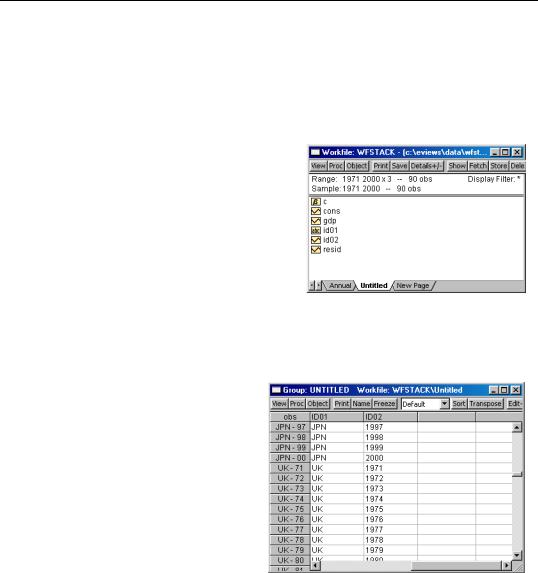
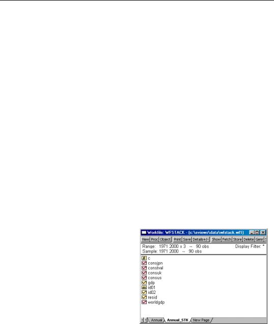
Here we see the resulting workfile page UNTITLED, containing the stacked series GDP and CONS, as well as two EViews created series objects, ID01 and ID02, that contain identifiers that may be used to structure the workfile.
ID01 is an alpha series that contains the stack ID values “US”, “UK”, and “JPN” which are used as group identifiers, and ID02 is a data series containing the year observation identifiers (more generally, ID02 will contain the values of the observation identifiers from the original page).
You may notice that EViews has already applied a panel structure to the page, so that there are three crosssections of annual data from 1971 to 2000, for a total of 90 observations.
Note that EViews will only apply a panel structure to the new page if we stack the data by series, but not if we interleave observations. Here, had we chosen to interleave, we would obtain a new 90 observation unstructured page containing the series GDP and CONS and the alpha ID01 and series ID02, with the observations for 1971 followed by observations for 1972, and so forth.
258—Chapter 9. Advanced Workfiles
We may add our individual series to the stacked series list, either directly by entering their names, or using wildcard expressions. We may use either of the stack series expressions:
gdp? cons? worldgdp constval
or
gdp? cons? *
to stack the various “GDP?” and “CONS?” series on top of each other, and the individual series WORLDGDP and CONSTVAL will be linked to the new page so that the original series values are repeatedly be stacked on top of themselves.
It is worth reminding you that the wildcard values for individual series are processed after the repeated measures series “GDP?” and “CONS?” are evaluated, so that a given series will only be used once. Thus, in the example above, the series CONSUS is used in forming the stacked CONS series, so that it is ignored when matching the individual series wildcard.
If we had instead entered the list
gdp? *
EViews would stack the various “GDP?” series on top of each other, and would also link the individual series CONSUS, CONSUK, CONSJPN, WORLDGDP, and CONSTVAL so that the values are stacked on top of themselves. In this latter case, the wildcard implies that since the series CONSUS is not used in forming a stacked repeated measures series, it is to be used as a stacked individual series.
Lastly, we note that since EViews will, by default, create a new page in the existing workfile, all individual series will be stacked or interleaved by creating link objects. If, for example, you enter the stack series list
gdp? cons? worldgdp constval
the series WORLDGDP and CONSTVAL will be linked to the destination page using the ID02 values. Alternately, if we
were to save the stacked data to a new workfile, by clicking on the Page Destination tab and entering appropriate values, EViews will copy the original WORLDGDP and CONSTVAL series to the new page, repeating the values of the original series in the stacked series.