Basic Panel Analysis

894—Chapter 28. Working with Panel Data

Alternately, selecting Individual cross-section graphs displays separate time series graphs for each cross-section, while Combined cross-section graphs displays separate lines for each cross-section in a single graph. We caution you that both types of panel graphs may become difficult to read when there are large numbers of cross-sections. For example, the individual graphs for the 10 cross-section panel data depicted here provides information on general trends, but little in the way of detail:

The remaining two options allow you to plot a single graph containing summary statistics for each period.

Basic Panel Analysis—895

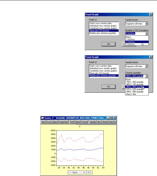
For line graphs, you may select Mean plus SD bounds, and then use the drop down menu on the lower right to choose between displaying no bounds, and 1, 2, or 3 standard deviation bounds. For other graph types such as area or spike, you may only display the means of the data by period.

For line graphs you may select Median plus extreme quantiles, and then use the drop down menu to choose additional extreme quantiles to be displayed. For other graph types, only the median may be plotted.

Suppose, for example, that we display a line graph containing the mean and 2 standard deviation bounds for the F series.

EViews computes, for each period, the mean and standard deviation of F across cross-sec- tions, and displays these in a time series graph:

Similarly, we may display a spike graph of the medians of F for each period:

896—Chapter 28. Working with Panel Data

Displaying graph views of a group object in a panel workfile involves similar choices about the handling of the panel structure.

Panel Unit Root Tests

EViews provides convenient tools for computing panel unit root tests. You may compute one or more of the following tests: Levin, Lin and Chu (2002), Breitung (2002), Im, Pesaran and Shin (2003), Fisher-type tests using ADF and PP tests—Maddala and Wu (1999) and Choi (2001), and Hadri (1999).

These tests are described in detail in “Panel Unit Root Tests” beginning on page 530.

To compute the unit root test on a series, simply select

View/Unit Root Test…from the menu of a series object.

By default, EViews will compute a Summary of all of the unit root tests, but you may use the combo box in the upper left hand corner to select an individual test statistic.

In addition, you may use the dialog to specify trend and intercept settings, to specify lag length selection, and to provide

details on the spectral estimation used in computing the test statistic or statistics.

898—Chapter 28. Working with Panel Data

Intermediate ADF test results

Estimation

EViews provides sophisticated tools for estimating equations in your panel structured workfile. See Chapter 29, “Panel Estimation”, beginning on page 901 for documentation.

Stacked By-Group Analysis

There are various by-group analysis tools that may be used to perform analysis of panel data. Previously, we considered an example of using by-group tools to examine data in “Cross-section and Period Summaries” on page 887. Standard by-group views may also be to test for equality of means, medians, or variances between groups, or to examine boxplots by cross-section or period.

For example, to compute a test of equality of means for F between firms, simply open the series, then select View/Test for Descriptive Statistics/Equality Tests by Classification....

Enter FN in the Series/Group for Classify edit field, and select OK to continue. EViews will compute and display the results for an ANOVA for F, classifying the data by firm ID. The top portion of the ANOVA results is given by:

Basic Panel Analysis—899

Test for Equality of Means of F

Categorized by values of FN

Date: 02/07/04 Time: 23:33

Sample: 1935 1954

Included observations: 200

Note in this example that we have relatively few cross-sections with moderate numbers of observations in each firm. Data with very large numbers of group identifiers and few observations are not recommended for this type of testing. To test equality of means between periods, call up the dialog and enter either YEAR or DATEID as the series by which you will classify.

A graphical summary of the primary information in the ANOVA may be obtained by displaying boxplots by cross-section or period. For moderate numbers of distinct classifier values, the graphical display may prove informative. Select View/

Descriptive Statistics/Boxplot by Classification... Enter FN in the Series/Group for Classify edit field, and select OK to display the boxplots using the default settings.

Stacked Analysis

A wide range of analyses are available in panel structured workfiles that have not been specifically redesigned to use the panel structure of your data. These tools allow you to

900—Chapter 28. Working with Panel Data

work with and analyze the stacked data, while taking advantage of the support for handling lags and leads in the panel structured workfile.

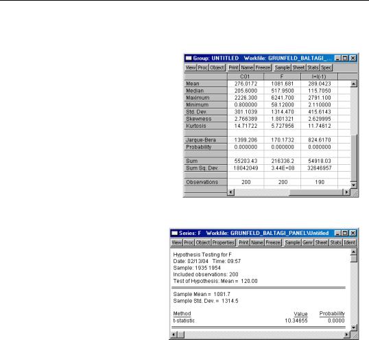
We may, for example, take our example panel workfile, create a group containing the series C01, F, and the expression I+I(-1), and then select

View/Descriptive Stats/Individual Samples from the group menu. EViews displays the descriptive statistics for the stacked data.

Note that the calculations are performed over the entire 200 observation stacked data, and that the statistics for I+I(-1) use only 190 observations (200 minus 10 observations corre-

sponding to the lag of the first observation for each firm).

Similarly, suppose you wish to perform a hypothesis testing on a single series. Open the window for the series F, and select View/Tests for Descriptive Stats/Simple Hypothesis Tests.... Enter “120” in the edit box for testing the mean value of the stacked series against a null of 120. EViews displays the results of a simple hypothesis test for the mean of the 200 observation stacked data.

While a wide variety of stacked analyses are supported, various views and procedures are not available in panel structured workfiles. You may not, for example, perform seasonal adjustment or estimate VAR or VEC models with the stacked panel.