712—Chapter 23. System Estimation
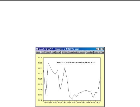
substitution between capital and labor is given by 1+c(3)/(C_K*C_L). Note that the elasticity of substitution is not a constant, and depends on the values of C_K and C_L. To create a series containing the elasticities computed for each observation, select Quick/ Generate Series…, and enter:
es_kl = 1 + sys1.c(3)/(c_k*c_l)
To plot the series of elasticity of substitution between capital and labor for each observation, double click on the series name ES_KL in the workfile and select View/Line Graph:
While it varies over the sample, the elasticity of substitution is generally close to one, which is consistent with the assumption of a Cobb-Douglas cost function.
Technical Discussion
While the discussion to follow is expressed in terms of a balanced system of linear equations, the analysis carries forward in a straightforward way to unbalanced systems containing nonlinear equations.
Denote a system of m equations in stacked form as:
|
|
|
|
|
|
|
|
|
|
|
|
|
|
y1 |
|
X1 0 … 0 |
|
β1 |
|
1 |
|
|
y2 |
= |
0 |
X2 |
|
|
β2 |
+ |
2 |
(23.4) |
|
|
|
|
|
0 |
|
|
|
|
|
|
yM |
|
0 |
… 0 XM |
|
βM |
|
M |
|
|
|
|
|
|
|
|
|
|
|
|
|
|
Technical Discussion—713
where ym is T vector, Xm is a T × km matrix, and βm is a km vector of coefficients. The error terms have an MT × MT covariance matrix V . The system may be written in compact form as:
Under the standard assumptions, the residual variance matrix from this stacked system is given by:
V = E( ′ ) = σ2( IM IT) . |
(23.6) |
Other residual structures are of interest. First, the errors may be heteroskedastic across the m equations. Second, they may be heteroskedastic and contemporaneously correlated. We can characterize both of these cases by defining the M × M matrix of contemporane-
ous correlations, Σ , where the (i,j)-th element of Σ is given by σij = E( it jt) for all |
t . If the errors are contemporaneously uncorrelated, then, σij |
= 0 for i ≠ j , and we can |
write: |
|
|
|
|
V = diag( σ2, σ2,…, σ |
2 |
) I |
T |
(23.7) |
1 2 |
M |
|
|
More generally, if the errors are heteroskedastic and contemporaneously correlated:
Lastly, at the most general level, there may be heteroskedasticity, contemporaneous correlation, and autocorrelation of the residuals. The general variance matrix of the residuals may be written:
|
σ11Σ11 |
σ12Σ12 |
… |
|
|
|
|
σ1MΣ1M |
|
|
σ21Σ21 |
σ22Σ22 |
|
|
|
(23.9) |
V = |
|
|
|
|
|
|
|
|
|
|
|
… |
|
|
|
|
σM1ΣM1 |
|
σMMΣMM |
|
where Σij is an autocorrelation matrix for the i-th and j-th equations.
Ordinary Least Squares
The OLS estimator of the estimated variance matrix of the parameters is valid under the assumption that V = Σ IT . The estimator for β is given by,
bLS = ( X′ X)−1X′y |
(23.10) |
and the variance estimator is given by: |
|
var( bLS) = s2( X′ X)−1 |
(23.11) |
where s2 is the residual variance estimate for the stacked system.
714—Chapter 23. System Estimation
Weighted Least Squares
The weighted least squares estimator is given by:
|
ˆ −1 |
X) |
−1 |
ˆ |
−1 |
(23.12) |
|
bWLS = ( X′V |
|
X′V |
y |
ˆ |
diag( s11, s22, …, sMM) IT is a consistent estimator of V , and sii is the |
where V = |
residual variance estimator, |
|
|
|
|
|
|
sij = ( ( yi − XibLS) ′( yj − XjbLS) ) ⁄ max( Ti, Tj) |
(23.13) |
where the inner product is taken over the non-missing common elements of i |
and j . The |
max function in Equation (23.13) is designed to handle the case of unbalanced data by down-weighting the covariance terms. Provided the missing values are asymptotically negligible, this yields a consistent estimator of the variance elements. Note also that there is no adjustment for degrees of freedom.
When specifying your estimation specification, you are given a choice of which coefficients to use in computing the sij . If you choose not to iterate the weights, the OLS coefficient estimates will be used to estimate the variances. If you choose to iterate the weights, the current parameter estimates (which may be based on the previously computed weights) are used in computing the sij . This latter procedure may be iterated until the weights and coefficients converge.
The estimator for the coefficient variance matrix is:
ˆ |
−1 |
−1 |
(23.14) |
var( bWLS) = ( X′V |
X) |
. |
The weighted least squares estimator is efficient, and the variance estimator consistent, under the assumption that there is heteroskedasticity, but no serial or contemporaneous correlation in the residuals.
It is worth pointing out that if there are no cross-equation restrictions on the parameters of the model, weighted LS on the entire system yields estimates that are identical to those obtained by equation-by-equation LS. Consider the following simple model:
y1 = X1β1 + 1
(23.15)
y2 = X2β2 + 2
If β1 and β2 are unrestricted, the WLS estimator given in Equation (23.14) yields:
b |
WLS |
= |
|
( ( X |
1′X |
1) ⁄ s11 )−1( ( X1′y1) ⁄ s11) |
|
= |
|
( X1′X1)−1X1′y1 |
|
. (23.16) |
|
|
|
|
|
( ( X2′X2) ⁄ s22 )−1( ( X2′y2) ⁄ s22) |
|
|
( X2′X2)−1X2′y2 |
|
|
|
|
|
|
|
|
|
|
|
|
|
|
|
|
|
|
|
|
|
|
|
|
|
|
|
The expression on the right is equivalent to equation-by-equation OLS. Note, however, that even without cross-equation restrictions, the standard errors are not the same in the two cases.

Technical Discussion—715
Seemingly Unrelated Regression (SUR)
SUR is appropriate when all the right-hand side regressors X are assumed to be exogenous, and the errors are heteroskedastic and contemporaneously correlated so that the error variance matrix is given by V = Σ IT . Zellner’s SUR estimator of β takes the form
ˆ |
−1 |
X ) |
−1 |
ˆ |
−1 |
(23.17) |
bSUR = ( X′( Σ IT) |
|
|
X′( Σ IT) |
y , |
ˆ
where Σ is a consistent estimate of Σ with typical element sij , for all i and j .
If you include AR terms in equation j , EViews transforms the model (see “Estimating AR Models” on page 497) and estimates the following equation:
|
pj |
|
+ jt |
|
yjt = Xjtβj + |
Σ ρjr( yj(t−r) − Xj(t−r)) |
(23.18) |
r = 1
where j is assumed to be serially independent, but possibly correlated contemporaneously across equations. At the beginning of the first iteration, we estimate the equation by nonlinear LS and use the estimates to compute the residuals ˆ . We then construct an estimate of Σ using sij = ( ˆi′ ˆj) ⁄ max( Ti, Tj) and perform nonlinear GLS to complete one iteration of the estimation procedure. These iterations may be repeated until the coefficients and weights converge.
Two-Stage Least Squares (TSLS) and Weighted TSLS
TSLS is a single equation estimation method that is appropriate when some of the variables in X are endogenous. Write the j-th equation of the system as,
YΓj + XBj + j |
= 0 |
(23.19) |
or, alternatively: |
|
|
|
|
|
yj = Yjγj + Xjβj + j |
= Zjδj + j |
(23.20) |
where Γj′ = ( −1, γj′, 0) , Bj′ |
= ( βj′, 0) , Zj′ = ( Yj′, Xj′) and δj′ |
= ( γj′, βj′) . Y |
is the matrix of endogenous variables and X is the matrix of exogenous variables. |
In the first stage, we regress the right-hand side endogenous variables yj |
on all exogenous |
variables X and get the fitted values: |
|
|
|
|
ˆ |
= X( X′X) |
−1 |
X′Xyj . |
(23.21) |
Yj |
|
In the second stage, we regress
ˆ ( ˆ ) where Zj = Yj, Xj .
ˆ |
|
|
to get: |
|
yj on Yj and Xj |
|
ˆ |
ˆ |
ˆ |
−1 ˆ |
(23.22) |
δ2SLS = |
( Zj′ Zj) |
Zj′y . |
716—Chapter 23. System Estimation
Weighted TSLS applies the weights in the second stage so that:
ˆ |
ˆ |
ˆ −1 |
ˆ |
−1 ˆ |
ˆ |
−1 |
(23.23) |
δW2SLS = |
( Zj′ V |
Zj) |
Zj′V |
y |
where the elements of the variance matrix are estimated in the usual fashion using the residuals from unweighted TSLS.
If you choose to iterate the weights, X is estimated at each step using the current values of the coefficients and residuals.
Three-Stage Least Squares (3SLS)
Since TSLS is a single equation estimator that does not take account of the covariances between residuals, it is not, in general, fully efficient. 3SLS is a system method that estimates all of the coefficients of the model, then forms weights and reestimates the model using the estimated weighting matrix. It should be viewed as the endogenous variable analogue to the SUR estimator described above.
The first two stages of 3SLS are the same as in TSLS. In the third stage, we apply feasible generalized least squares (FGLS) to the equations in the system in a manner analogous to the SUR estimator.
SUR uses the OLS residuals to obtain a consistent estimate of the cross-equation covariance matrix Σ . This covariance estimator is not, however, consistent if any of the righthand side variables are endogenous. 3SLS uses the 2SLS residuals to obtain a consistent estimate of Σ .
In the balanced case, we may write the equation as,
ˆ |
ˆ |
−1 |
X( X′X) |
−1 |
X′ ) Z) |
−1 |
ˆ |
−1 |
X( X′X) |
−1 |
X′) y , (23.24) |
δ3SLS = ( Z( Σ |
|
|
Z |
( Σ |
|
|
ˆ |
|
|
|
|
|
|
|
|
|
|
|
where Σ has typical element: |
|
|
|
|
|
|
|
|
sij |
|
|
ˆ |
|
ˆ |
|
|
|
|
|
(23.25) |
= ( ( yi − Ziγ2SLS) ′( yj − Zjγ2SLS) ) ⁄ max( Ti, Tj) . |
|
If you choose to iterate the weights, the current coefficients and residuals will be used to
ˆ
estimate Σ .
Generalized Method of Moments (GMM)
The basic idea underlying GMM is simple and intuitive. We have a set of theoretical moment conditions that the parameters of interest θ should satisfy. We denote these moment conditions as:
E( m( y, θ) ) = 0 . |
(23.26) |
The method of moments estimator is defined by replacing the moment condition (23.26) by its sample analog:
|
Technical Discussion—717 |
|
|
( Σ m( yt, θ) ) ⁄ T = 0 . |
(23.27) |
t |
|
However, condition (23.27) will not be satisfied for any θ when there are more restrictions m than there are parameters θ . To allow for such overidentification, the GMM estimator is defined by minimizing the following criterion function:
Σm( yt, θ) A( yt, θ)m( yt, θ) |
(23.28) |
t |
|
which measures the “distance” between m and zero. A is a weighting matrix that weights each moment condition. Any symmetric positive definite matrix A will yield a consistent estimate of θ . However, it can be shown that a necessary (but not sufficient) condition to obtain an (asymptotically) efficient estimate of θ is to set A equal to the inverse of the covariance matrix Ω of the sample moments m . This follows intuitively, since we want to put less weight on the conditions that are more imprecise.
To obtain GMM estimates in EViews, you must be able to write the moment conditions in Equation (23.26) as an orthogonality condition between the residuals of a regression equation, u( y, θ, X) , and a set of instrumental variables, Z , so that:
m( θ, y, X, Z ) = Z′u( θ, y, X) |
(23.29) |
For example, the OLS estimator is obtained as a GMM estimator with the orthogonality conditions:
X′( y − Xβ) = 0 . |
(23.30) |
For the GMM estimator to be identified, there must be at least as many instrumental variables Z as there are parameters θ . See the section on “Generalized Method of Moments (GMM)” beginning on page 488 for additional examples of GMM orthogonality conditions.
An important aspect of specifying a GMM problem is the choice of the weighting matrix |
A . EViews uses the optimal A = |
ˆ |
−1 |
ˆ |
Ω |
|
, where Ω is the estimated covariance matrix of |
the sample moments m . EViews uses the consistent TSLS estimates for the initial estimate of θ in forming the estimate of Ω .
White’s Heteroskedasticity Consistent Covariance Matrix
If you choose the GMM-Cross section option, EViews estimates Ω using White’s heteroskedasticity consistent covariance matrix:
ˆ |
ˆ |
1 |
|
T |
Z |
′u |
u |
′Z |
|
(23.31) |
ΩW = Γ( 0) = |
------------ |
|
Σ |
t |
|
|
T − k |
t |
t |
t |
|
|
|
|
|
|
t = 1 |
|
|
|
|
|
|
where u is the vector of residuals, and Zt is a k × p matrix such that the p moment conditions at t may be written as m( θ, yt, Xt, Zt) = Zt′u( θ, yt, Xt) .
718—Chapter 23. System Estimation
Heteroskedasticity and Autocorrelation Consistent (HAC) Covariance
Matrix
If you choose the GMM-Time series option, EViews estimates Ω by,
ˆ |
|
ˆ |
T − 1 |
|
|
ˆ |
|
|
ˆ |
|
|
ΩHAC |
= Γ( 0) + Σ k( j, q)( Γ( j) + Γ |
′( j) ) |
|
|
|
|
j = 1 |
|
|
|
|
|
|
|
|
where: |
|
|
|
|
|
|
|
|
|
|
|
|
ˆ |
|
1 |
|
T |
|
|
′u |
|
|
′Z |
|
|
|
|
Z |
|
u |
|
. |
Γ( j) |
= ------------ |
Σ |
t − j |
t − j |
t |
|
|
T − k |
|
t |
|
|
|
|
|
|
|
t = j + 1 |
|
|
|
|
|
|
|
|
You also need to specify the kernel κ and the bandwidth q .
Kernel Options
ˆ
The kernel κ is used to weight the covariances so that Ω is ensured to be positive semidefinite. EViews provides two choices for the kernel, Bartlett and quadratic spectral (QS). The Bartlett kernel is given by,
κ( j, q) |
|
1 − ( j ⁄ q) |
0 ≤ j ≤ q |
= |
0 |
otherwise |
|
|
while the quadratic spectral (QS) kernel is given by:
k( j ⁄ q) |
= |
25 |
|
sin( 6πx ⁄ 5) |
|
------------------- |
2- |
|
----------------------------- − cos ( 6πx ⁄ 5 ) |
|
|
12( πx) |
6πx ⁄ 5 |
|
|
|
|
|
|
|
where x = j ⁄ q . The QS has a faster rate of convergence than the Bartlett and is smooth and not truncated (Andrews 1991). Note that even though the QS kernel is not truncated, it still depends on the bandwidth q (which need not be an integer).
Bandwidth Selection
The bandwidth q determines how the weights given by the kernel change with the lags in the estimation of Ω . Newey-West fixed bandwidth is based solely on the number of observations in the sample and is given by:
q = int( 4( T ⁄ 100)2 ⁄ 9) |
(23.36) |
where int( ) denotes the integer part of the argument.
EViews also provides two “automatic”, or data dependent bandwidth selection methods that are based on the autocorrelations in the data. Both methods select the bandwidth according to:
|
|
|
|
|
|
|
Technical Discussion—719 |
|
|
|
|
|
|
|
|
|
|
ˆ |
|
|
1 ⁄ 3 |
) |
for the Bartlett kernel |
int( 1.1447 ( α( 1) T) |
|
q = |
|
ˆ |
|
1 ⁄ 5 |
|
(23.37) |
|
1.3221 |
2 )T) |
|
for the QS kernel |
|
( α( |
|
|
|
|
The two methods, Andrews and Variable-Newey-West, differ in how they estimate αˆ ( 1) and αˆ ( 2 ) .
Andrews (1991) is a parametric method that assumes the sample moments follow an AR(1) process. We first fit an AR(1) to each sample moment (23.29) and estimate the auto-
ˆ |
ˆ 2 |
for i = 1, 2, …, zn , where z |
correlation coefficients ρi |
and the residual variances σi |
is the number of instrumental variables and n is the number of equations in the system.
ˆ |
ˆ |
|
|
|
|
|
|
|
|
|
|
|
|
|
|
|
|
Then α( 1) |
and α( 2 ) are estimated by: |
|
|
|
|
|
|
|
|
|
|
|
|
|
ˆ |
|
zn |
|
ˆ 2 |
ˆ |
4 |
|
|
|
zn |
ˆ |
4 |
|
|
|
|
4ρi |
σi |
|
|
|
σi |
|
α( 1 ) = |
|
Σ |
------------------------------------------- |
⁄ |
Σ |
-------------------- |
|
|
|
|
ˆ |
6 |
( |
|
|
ˆ |
2 |
|
|
ˆ |
4 |
|
|
i = 1 |
( 1 − ρi) |
|
1 + ρi) |
i = 1 ( 1 − |
ρi) |
|
|
|
|
ˆ 2 |
ˆ 4 |
|
|
|
|
|
ˆ 4 |
|
|
|
|
(23.38) |
|
ˆ |
zn |
|
zn |
|
|
|
|
|
|
|
4ρi |
σi |
⁄ |
|
|
σi |
|
|
|
|
|
α( 2 ) = |
|
Σ |
-------------------- |
|
Σ |
-------------------- |
|
|
|
|
|
|
ˆ |
8 |
|
|
|
( 1 |
ˆ |
|
4 |
|
|
|
|
i = 1 |
( 1 − ρi) |
|
|
i = 1 |
− ρi) |
|
|
|
|
Note that we weight all moments equally, including the moment corresponding to the constant.
Newey-West (1994) is a nonparametric method based on a truncated weighted sum of the
|
ˆ |
ˆ |
ˆ |
( 2 ) are estimated by, |
|
|
estimated cross-moments Γ( j) . |
α( 1 ) and α |
|
|
|
ˆ |
l′F( p) l |
(23.39) |
|
|
α( p) = |
----------------- |
|
|
|
l′F( 0) l |
|
|
where l is a vector of ones and: |
|
|
|
|
|
|
|
|
F( p) = Γ( 0) + |
L |
|
p |
ˆ |
ˆ |
|
|
Σ i |
(23.40) |
|
|
( Γ |
( i) + Γ′( i) ) , |
i = 1
for p = 1, 2 .
One practical problem with the Newey-West method is that we have to choose a lag selection parameter L . The choice of L is arbitrary, subject to the condition that it grow at a certain rate. EViews sets the lag parameter to
int( 4( T ⁄ 100)2 ⁄ 9) |
for the Bartlett kernel |
L = |
|
(23.41) |
|
T |
for the QS kernel |
720—Chapter 23. System Estimation
Prewhitening
You can also choose to prewhiten the sample moments m to “soak up” the correlations in m prior to GMM estimation. We first fit a VAR(1) to the sample moments:
mt |
= Amt − 1 + vt . |
|
|
|
|
|
(23.42) |
ˆ |
ˆ |
− A ) |
−1 ˆ |
|
( I − A ) |
−1 |
ˆ |
|
is |
Then the variance Ω of m is estimated by Ω = ( I |
Ω |
|
|
where Ω |
|
the variance of the residuals vt and is computed using any of the above methods. The GMM estimator is then found by minimizing the criterion function:
Note that while Andrews and Monahan (1992) adjust the VAR estimates to avoid singularity when the moments are near unit root processes, EViews does not perform this eigenvalue adjustment.