

326—Chapter 11. Series
Correlogram
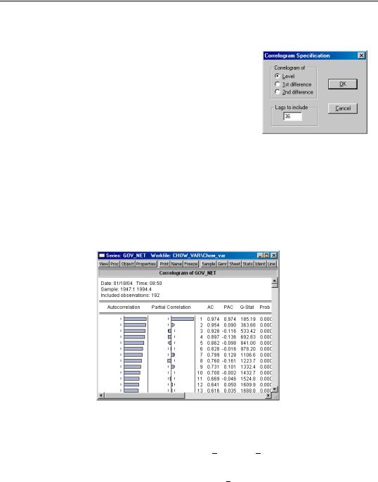
This view displays the autocorrelation and partial autocorrelation functions up to the specified order of lags. These functions characterize the pattern of temporal dependence in the series and typically make sense only for time series data. When you select View/Correlogram… the Correlogram Specification dialog box appears.
You may choose to plot the correlogram of the raw series (level) x, the first difference d(x)=x–x(–1), or the second difference
d(x)-d(x(-1)) = x-2x(-1)+x(-2)
of the series.
You should also specify the highest order of lag to display the correlogram; type in a positive integer in the field box. The series view displays the correlogram and associated statistics:
Autocorrelations (AC)
The autocorrelation of a series Y at lag k is estimated by:
T
Σ ( Yt − Y) ( Yt − k − Y)
τ = t = k + 1
k ---------------------------------------------------------------- (11.15)
T
Σ ( Yt − Y)2
t = 1

Correlogram—327
where Y is the sample mean of Y . This is the correlation coefficient for values of the series k periods apart. If τ1 is nonzero, it means that the series is first order serially correlated. If τk dies off more or less geometrically with increasing lag k , it is a sign that the series obeys a low-order autoregressive (AR) process. If τk drops to zero after a small number of lags, it is a sign that the series obeys a low-order moving-average (MA) process. See “Serial Correlation Theory” on page 493 for a more complete description of AR and MA processes.
Note that the autocorrelations estimated by EViews differ slightly from theoretical descriptions of the estimator:
T
Σ ( ( Yt − Y )( Yt − k − Y) ) ⁄ ( T − K )
τk = t--------------------------------------------------------------------------------------------= k + 1 |
T |
(11.16) |
||
|
Σ ( Yt − |
|
)2 ⁄ T |
|
|
Y |
|
||
|
t = 1 |
|
||
where Yt − k = ΣYt − k ⁄ ( T − k) . The difference arises since, for computational simplicity, EViews employs the same overall sample mean Y as the mean of both Yt and Yt − k . While both formulations are consistent estimators, the EViews formulation biases the result toward zero in finite samples.
The dotted lines in the plots of the autocorrelations are the approximate two standard error bounds computed as ±2 ⁄ ( T ) . If the autocorrelation is within these bounds, it is not significantly different from zero at (approximately) the 5% significance level.
Partial Autocorrelations (PAC)
The partial autocorrelation at lag k is the regression coefficient on Yt − k when Yt is regressed on a constant, Yt − 1, …, Yt − k . This is a partial correlation since it measures the correlation of Y values that are k periods apart after removing the correlation from the intervening lags. If the pattern of autocorrelation is one that can be captured by an autoregression of order less than k , then the partial autocorrelation at lag k will be close to zero.
The PAC of a pure autoregressive process of order p , AR( p ), cuts off at lag p , while the PAC of a pure moving average (MA) process asymptotes gradually to zero.
EViews estimates the partial autocorrelation at lag k recursively by

328—Chapter 11. Series
|
|
|
|
τ1 |
|
for k = 1 |
|
|
|
|
|
|
|
||
|
|
|
|
|
k − 1 |
|
|
φ |
|
= |
|
τk − |
Σ φk − 1, j τk − j |
|
(11.17) |
|
k |
|
|
|
j = 1 |
for k > 1 |
|
|
|
|
|
------------------------------------------------- |
|
||
|
|
|
|
|
k − 1 |
|
|
|
|
|
1 − |
Σ φk − 1, j τk − j |
|
|
|
|
|
|
|
|
j = 1 |
|
|
where τk is the estimated autocorrelation at lag k and where, |
|
||||||
|
|
|
φk, j = φk − 1, j − φkφk − 1, k − j. |
(11.18) |
|||
This is a consistent approximation of the partial autocorrelation. The algorithm is described in Box and Jenkins (1976, Part V, Description of computer programs). To obtain a more precise estimate of φ , simply run the regression:
Yt = β0 + β1Yt − 1 + … + βk − 1Yt − (k − 1) + φkYt − k + et |
(11.19) |
where et is a residual. The dotted lines in the plots of the partial autocorrelations are the approximate two standard error bounds computed as ± 2 ⁄ ( T ) . If the partial autocorrelation is within these bounds, it is not significantly different from zero at (approximately) the 5% significance level.
Q-Statistics
The last two columns reported in the correlogram are the Ljung-Box Q-statistics and their p-values. The Q-statistic at lag k is a test statistic for the null hypothesis that there is no autocorrelation up to order k and is computed as:
|
k |
2 |
|
|
QLB = T( T + 2 ) |
τj |
|
||
Σ |
(11.20) |
|||
------------ |
||||
|
T − J |
|
||
|
j = 1 |
|
|
where τj is the j-th autocorrelation and T is the number of observations. If the series is not based upon the results of ARIMA estimation, then under the null hypothesis, Q is asymptotically distributed as a χ2 with degrees of freedom equal to the number of autocorrelations. If the series represents the residuals from ARIMA estimation, the appropriate degrees of freedom should be adjusted to represent the number of autocorrelations less the number of AR and MA terms previously estimated. Note also that some care should be taken in interpreting the results of a Ljung-Box test applied to the residuals from an ARMAX specification (see Dezhbaksh, 1990, for simulation evidence on the finite sample performance of the test in this setting).
The Q-statistic is often used as a test of whether the series is white noise. There remains the practical problem of choosing the order of lag to use for the test. If you choose too small a lag, the test may not detect serial correlation at high-order lags. However, if you
Unit Root Test—329
choose too large a lag, the test may have low power since the significant correlation at one lag may be diluted by insignificant correlations at other lags. For further discussion, see Ljung and Box (1979) or Harvey (1990, 1993).
Unit Root Test
This view carries out the Augmented Dickey-Fuller (ADF), GLS transformed Dickey-Fuller (DFGLS), Phillips-Perron (PP), Kwiatkowski, et. al. (KPSS), Elliot, Richardson and Stock (ERS) Point Optimal, and Ng and Perron (NP) unit root tests for whether the series (or it’s first or second difference) is stationary.
See “Nonstationary Time Series” on page 517 for a discussion of stationary and nonstationary time series and additional details on how to carry out the unit roots tests in Eviews.
BDS Test
This view carries out the BDS test for independence, as described in Brock, Dechert, Scheinkman and LeBaron (1996).
The BDS test is a portmanteau test for time based dependence in a series. It can be used for testing against a variety of possible deviations from independence including linear dependence, non-linear dependence, or chaos.
The test can be applied to a series of estimated residuals to check whether the residuals are independent and identically distributed (iid). For example, the residuals from an ARMA model can be tested to see if there is any non-linear dependence in the series after the linear ARMA model has been fitted.
The idea behind the test is fairly simple. To perform the test, we first choose a distance, . We then consider a pair of points. If the observations of the series truly are iid, then for any pair of points, the probability of the distance between these points being less than or equal to epsilon will be constant. We denote this probability by c1( ) .
We can also consider sets consisting of multiple pairs of points. One way we can choose sets of pairs is to move through the consecutive observations of the sample in order. That is, given an observation s , and an observation t of a series X, we can construct a set of pairs of the form:
{{Xs, Xt} , {Xs + 1, Xt + 1} , {Xs + 2, Xt + 2} , …, {Xs + m − 1, Xt + m − 1} } (11.21)
where m is the number of consecutive points used in the set, or embedding dimension. We denote the joint probability of every pair of points in the set satisfying the epsilon condition by the probability cm( ) .

330—Chapter 11. Series
The BDS test proceeds by noting that under the assumption of independence, this probability will simply be the product of the individual probabilities for each pair. That is, if the observations are independent,
cm( ) = c1m( ) . |
(11.22) |
When working with sample data, we do not directly observe c1( ) or cm( ) . We can only estimate them from the sample. As a result, we do not expect this relationship to hold exactly, but only with some error. The larger the error, the less likely it is that the error is caused by random sample variation. The BDS test provides a formal basis for judging the size of this error.
To estimate the probability for a particular dimension, we simply go through all the possible sets of that length that can be drawn from the sample and count the number of sets which satisfy the condition. The ratio of the number of sets satisfying the condition divided by the total number of sets provides the estimate of the probability. Given a sample of n observations of a series X, we can state this condition in mathematical notation,
|
|
2 |
n − m + 1 n − m + 1 m − 1 |
|
|||||
cm, n( ) |
= |
|
Σ |
|
Σ |
|
Π I (Xs + j, Xt + j ) |
(11.23) |
|
(--------------------------------------------------n − m + 1) ( n − m) |
|
|
|||||||
|
|
s = 1 t = s + 1 j = 0 |
|
||||||
|
|
|
|
|
|||||
where I is the indicator function: |
|
|
|
|
|
|
|
||
|
|
|
1 |
if |
|
x − y |
|
≤ |
|
|
|
|
|
|
|||||
|
|
I (x, y ) = |
|
|
(11.24) |
||||
|
|
0 |
otherwise. |
|
|||||
Note that the statistics cm, n are often referred to as correlation integrals.
We can then use these sample estimates of the probabilities to construct a test statistic for independence:
b |
( ) = c |
( ) − c |
( )m |
(11.25) |
|
m, n |
m, n |
1, n − m + 1 |
|
where the second term discards the last m − 1 observations from the sample so that it is based on the same number of terms as the first statistic.
Under the assumption of independence, we would expect this statistic to be close to zero. In fact, it is shown in Brock et al. (1996) that
|
|
|
|
( |
|
bm, n( ) |
→ N( 0, 1 ) |
|
|
|
|||||
|
|
|
|
n − m + 1) ------------------ |
|
|
|
||||||||
|
|
|
|
|
|
σm, n( ) |
|
|
|
|
|
|
|||
where |
|
|
|
|
|
|
|
|
|
|
|
|
|
|
|
2 |
|
|
|
m |
m − 1 |
m − j |
|
2j |
|
2 |
|
2m |
2 |
|
2m − 2 |
σm, n( ) |
= |
4 |
k |
|
+ 2 Σ k |
|
c1 |
|
+ ( m − 1) |
c |
1 |
− m |
kc1 |
|
|
j = 1
(11.26)
(11.27)
BDS Test—331
and where c1 can be estimated using c1, n . k is the probability of any triplet of points lying within of each other, and is estimated by counting the number of sets satisfying the sample condition:
kn( ) |
|
2 |
n |
n |
n |
|
= |
n--------------------------------------( n − 1 ) -( n − 2) Σ Σ Σ |
(11.28) |
||||
|
|
|
||||
|
|
|
t = 1 s = t + 1 r = s + 1 |
|
||
( I (Xt, Xs)I (Xs, Xr) + I (Xt, Xr)I (Xr, Xs) + I (Xs, Xt)I (Xt, Xr))
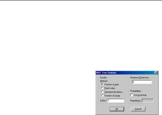
To calculate the BDS test statistic in EViews, simply open the series you would like to test in a window, and choose View/BDS Independence Test.... A dialog will appear prompting you to input options.
To carry out the test, we must choose , the distance used for testing proximity of the data points, and the dimension m , the number of consecutive data points to include in the set.
The dialog provides several choices for how to specify :
•Fraction of pairs: is calculated so as to ensure a certain fraction of the total number of pairs of points in the sample lie within of each other.
•Fixed value: is fixed at a raw value specified in the units as the data series.
•Standard deviations: is calculated as a multiple of the standard deviation of the series.
•Fraction of range: is calculated as a fraction of the range (the difference between the maximum and minimum value) of the series.
The default is to specify as a fraction of pairs, since this method is most invariant to different distributions of the underlying series.
You must also specify the value used in calculating . The meaning of this value varies based on the choice of method. The default value of 0.7 provides a good starting point for the default method when testing shorter dimensions. For testing longer dimensions, you should generally increase the value of to improve the power of the test.
EViews also allows you to specify the maximum correlation dimension for which to calculate the test statistic. EViews will calculate the BDS test statistic for all dimensions from 2 to the specified value, using the same value of or each dimension. Note the same is