


Chapter 5. Basic Data Handling
The process of entering, reading, editing, manipulating, and generating data forms the foundation of most data analyses. Accordingly, most of your time in EViews will probably be spent working with data. EViews provides you with a sophisticated set of data manipulation tools that make these tasks as simple and straightforward as possible.
This chapter describes the fundamentals of working with data in EViews. There are three cornerstones of data handling in EViews: the two most common data objects, series and groups, and the use of samples which define the set of observations in the workfile that we wish to use in analysis.
We begin our discussion of data handling with a brief description of series, groups, and samples, and then discuss the use of these objects in basic input, output, and editing of data. Lastly, we describe the basics of frequency conversion.
In Chapter 6, “Working with Data”, on page 129, we discuss the basics of EViews’ powerful language for generating and manipulating the data held in series and groups. Subsequent chapters describe additional techniques and objects for working with data.
Data Objects
The actual numeric values that make up your data will generally be held in one or more of EViews’ data objects (series, groups, matrices, vectors, and scalars). For most users, series and groups will by far be the most important objects, so they will be the primary focus of our discussion. Matrices, vectors, and scalars are discussed at greater length in the Command and Programming Reference.
The following discussion is intended to provide only a brief introduction to the basics of series and groups. Our goal is to describe the fundamentals of data handling in EViews. An in-depth discussion of series and group objects follows in subsequent chapters.
Series
An EViews series contains a set of observations on a numeric variable. Associated with each observation in the series is a date or observation label. For series in dated workfiles, the observations are presumed to be observed regularly over time. For undated data, the observations are not assumed to follow any particular frequency.
Note that the series object may only be used to hold numeric data. If you wish to work with alphanumeric data, you should employ alpha series. See “Alpha Series” on page 153 for discussion.
88—Chapter 5. Basic Data Handling
Creating a series
One method of creating a numeric series is to select Object/New Object… from the menu, and then to select Series. You may, at this time, provide a name for the series, or you can let the new series be untitled. Click OK. EViews will open a spreadsheet view of the new series object. All of the observations in the series will be assigned the missing value code “NA”. You can then edit or use expressions to assign values for the series.
You may also use the New Object dialog to create alpha series. Alpha series are discussed in greater detail in “Alpha Series” on page 153.
The second method of creating a series is to generate the series using mathematical expressions. Click on Quick/Generate Series… in the main EViews menu, and enter an expression defining the series. We will discuss this method in depth in the next chapter.
Changing the Spreadsheet Display
EViews provides you with extensive ability to customize your series spreadsheet display.
Column Widths
To resize the width of a column, simply move your mouse over the column separator and until the icon changes, then drag the column to its desired width. The new width will be remembered the next time you open the series and will be used when the series is displayed in a group spreadsheet.
Display Type
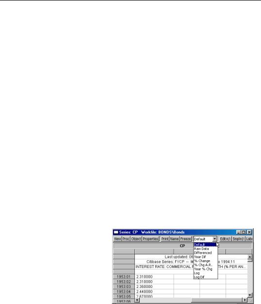
The series display type, which is listed in the combo box in the series toolbar, determines how the series spreadsheet window shows your data.
The Default method shows data in either raw (underlying data) form or, if a value map is attached to the series, shows the mapped values. Alternatively, you may use the Raw Data to show only the underlying data. See “Value Maps” on page 163 for a description of the use of value maps.
Data Objects—89
You may also use the display type setting to show transformations of the data. You may, for example, set the display method to Differenced, in order to have EViews display the firstdifferences of your data.
Changing the display of your series values does not alter the underlying values in the series,
it only modifies the values shown in the spreadsheet (the series header, located above the labels, will also change to indicate the transformation). Note, however, that if you edit the values of your series while displayed in transformed mode, EViews will change the underlying values of the series accordingly. Changing the display and editing data in transformed mode is a convenient method of inputting data that arrive as changes or other transformed values.
Display Formats
You may customize the way that numbers or characters in your series are displayed in the spreadsheet by setting the series display properties. To display the dialog, either select View/Properties from the series menu, click on Properties in the series toolbar, or right mouse click and select the Display Format... entry in the menu.
EViews will open the Properties dialog with the Display tab selected. You should use this dialog to change the default column width and justification for the series, and to choose from a large list of numeric display formats.
You may, for example, elect to change the display of numbers to show additional digits, to separate thousands with a comma, or to display numbers as fractions. The last four items in the Numeric display combo box provide options for the formatting of date number.
Similarly, you may elect to change the series justification by selecting Auto, Left, Center, or Right. Note that Auto justification will set justification to right for numeric series, and left for alpha series.
90—Chapter 5. Basic Data Handling
You may also use this dialog to change the column width (note that column widths in spreadsheets may also be changed interactively by dragging the column headers).
Once you click on OK, EViews will accept the current settings and change the spreadsheet display to reflect your choices. In addition, these display settings will be used whenever the series spreadsheet is displayed or as the default settings when the series is used in a group spreadsheet display.
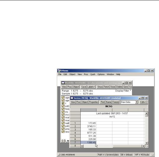
Note that when you apply a display format, you may find that a portion of the contents of a cell are not visible, when, for example, the column widths are too small to show the entire cell. Alternately, you may have a numeric cell for which the current display format only shows a portion of the full precision value.
In these cases, it may be useful to examine the actual contents of a table cell. To do so, simply select the table cell. The unformatted contents of the cell will appear in the status line at the bottom of the EViews window.
Narrow versus Wide
The narrow display displays the observations for the series in a single column, with date labels in the margin. The typical series spreadsheet display will use this display format.
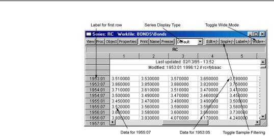
The wide display arranges the observations from left to right and top to bottom, with the label for the first observation in the row displayed in the margin. For dated workfiles, EViews will, if possible, arrange the data in a form which matches the frequency of the data. Thus, semi-annual data will be displayed with two observations per row, quarterly data will contain four observations per row, and 5-day daily data will contain five observations in each row.
Data Objects—91
You can change the display to show the observations in your series in multiple columns by clicking on the
Wide +/- button on the spreadsheet view toolbar (you may need to resize the series window to make this button visible). For example, toggling the
Wide +/- button
switches the display between the wide display (as depicted), and the narrow (single column) display.
This wide display format is useful when you wish to arrange observations for a particular season in each of the columns.
Sample Subset Display
By default, all observations in the workfile are displayed, even those observations not in the current sample. By pressing Smpl +/– you can toggle between showing all observations in the workfile, and showing only those observations included in the current sample.
There are two features that you should keep in mind as you toggle between the various display settings:
•If you choose to display only the observations in the current sample, EViews will switch to single column display.
•If you switch to wide display, EViews automatically turns off the display filter so that all observations in the workfile are displayed.
One consequence of this behavior is that if you begin with a narrow display of observations in the current sample, click on Wide +/- to switch to wide display, and then press the Wide +/- button again, EViews will provide a narrow display of all of the observations in the workfile. To return to the original narrow display of the current sample, you will need to press the Smpl +/- button again.
Editing a series
You can edit individual values of the data in a series.
92—Chapter 5. Basic Data Handling
First, open the spreadsheet view of the series. If the series window display does not show the spreadsheet view, click on the Sheet button, or select View/Spreadsheet, to change the default view.
Next, make certain that the spreadsheet window is in edit mode. EViews provides you with the option of protecting the data in your series by turning off the ability to edit from the spreadsheet window. You can use the Edit +/– button on the toolbar to toggle between edit mode and protected mode.
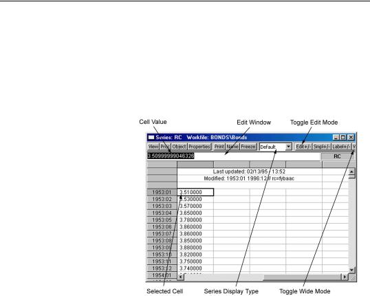
Here we see a series spreadsheet window in edit mode. Notice the presence of the edit window just beneath the series toolbar containing the value of RC in 1953M01, and the box around the selected cell in the spreadsheet; neither are present in protected mode.
To change the value for an observation, select the cell, type in the value, and press ENTER. For exam-
ple, to change the value of RC in 1953M01, simply click on the cell containing the value, type the new value in the edit window, and press ENTER.
When editing series values, you should pay particular attention to the series display format, which tells you the units in which your series are displayed. Here, we see that the series values are displayed in Default mode so that you are editing the underlying series values (or their value mapped equivalents). Alternately, if the series were displayed in Differenced mode, then the edited values correspond to the first differences of the series.
Note that some cells in the spreadsheet are protected. For example, you may not edit the observation labels, or the “Last update” series label. If you select one of the protected cells, EViews will display a message in the edit window telling you that the cell cannot be edited.
When you have finished editing, you should protect yourself from inadvertently changing values of your data by clicking on Edit +/– to turn off edit mode.

Data Objects—93
Inserting and deleting observations in a series
You can also insert and delete observations in the series. To insert an observation, first click on the cell where you want the new observation to appear. Next, click on the InsDel button on the series toolbar (you may have to expand the window to make this button visible). You will see a dialog asking whether you wish to insert or delete an observation at the current position.
If you choose to insert an observation, EViews will insert a missing value at the appropriate position and push all of the observations down so that the last observation will be lost from the workfile. If you wish to preserve this observation, you will have to expand the workfile before inserting observations. If you
choose to delete an observation, all of the remaining observations will move up, so that you will have a missing value at the end of the workfile range.
Groups
When working with multiple series, you will often want to create a group object to help you manage your data. A group is a list of series names (and potentially, mathematical expressions) that provides simultaneous access to all of the elements in the list.
With a group, you can refer to sets of variables using a single name. Thus, a set of variables may be analyzed, graphed, or printed using the group object, rather than each one of the individual series. Therefore, groups are often used in place of entering a lengthy list of names. Once a group is defined, you can use the group name in many places to refer to all of the series contained in the group.
You will also create groups of series when you wish to analyze or examine multiple series at the same time. For example, groups are used in computing correlation matrices, testing for cointegration and estimating a VAR or VEC, and graphing series against one another.
Creating Groups
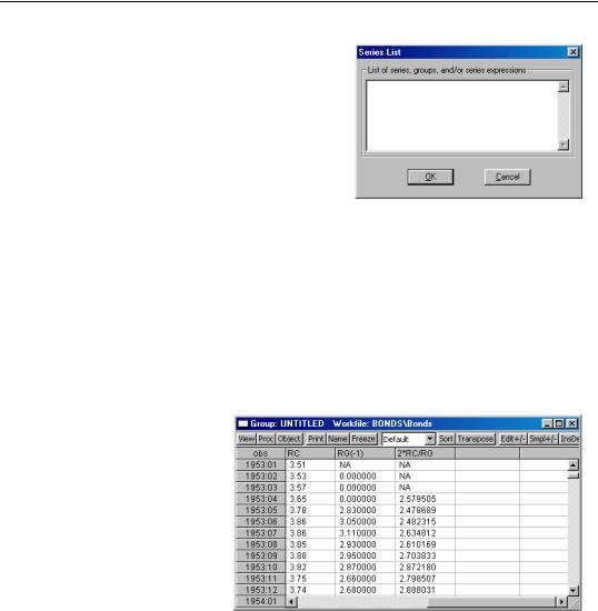
There are several ways to create a group. Perhaps the easiest method is to select Object/ New Object… from the main menu or workfile toolbar, click on Group, and if desired, name the object.
94—Chapter 5. Basic Data Handling
You should enter the names of the series to be included in the group, separated by spaces, and then click OK. A group window will open showing a spreadsheet view of the group.
You may have noticed that the dialog allows you to use group names and series expressions. If you include a group name, all of the series in the named group will be included in the new group. For example, suppose that the group GR1 con-
tains the series X, Y, and Z, and you create a new group GR2, which contains GR1 and the series A and B. Then GR2 will contain X, Y, Z, A and B. Bear in mind that only the series contained in GR1, not GR1 itself, are included in GR2; if you later add series to GR1, they will not be added to GR2.
Series expressions will be discussed in greater depth later. For now, it suffices to note that series expressions are mathematical expressions that may involve one or more series (e.g. “7/2” or “3*X*Y/Z”). EViews will automatically evaluate the expressions for each observation and display the results as if they were an ordinary series. Users of spreadsheet programs will be familiar with this type of automatic recalculation.
Here, for example, is a spreadsheet view of an untitled group containing the series RC, a series expression for the lag of RG, RG(– 1), and a series expression involving RC and RG.
Notice here the Default setting for the group spreadsheet display indicates that the series RC and RG(-1) are
displayed using the original values, spreadsheet types, and formats set in the original series (see “Display Formats” on page 89). A newly created group always uses the Default display setting, regardless of the settings in the original series, but the group does adopt the original series cell formatting. You may temporarily override the display setting by selecting a group display format. For example, to use the display settings of the original series, you should select Series Spec; to display differences of all of the series in the group, select Differenced.
An equivalent method of creating a group is to select Quick/Show…, or to click on the Show button on the workfile toolbar, and then to enter the list of series, groups and series