Добавил:
Upload Опубликованный материал нарушает ваши авторские права? Сообщите нам.
Вуз: Предмет: Файл:
Eviews5 / EViews5 / Docs / EViews 5 Users Guide.pdf
Скачиваний:
152
Добавлен:
23.03.2015
Размер:
11.51 Mб
Скачать

Chapter 29. Panel Estimation

EViews allows you to estimate panel equations using linear or nonlinear squares or instrumental variables (two-stage least squares), with correction for fixed or random effects in both the cross-section and period dimensions, AR errors, GLS weighting, and robust standard errors. In addition, GMM tools may be used to estimate most of the these specifications with various system-weighting matrices. Specialized forms of GMM also allow you to estimate dynamic panel data specifications. Note that all of the estimators described in this chapter require a panel structured workfile (“Structuring a Panel Workfile” on page 873).

We begin our discussion by briefly outlining the dialog settings associated with common panel equation specifications. While the wide range of models that EViews supports means that we cannot exhaustively describe all of the settings and specifications, we hope to provide you a roadmap of the steps you must take to estimate your panel equation.

More useful, perhaps, is the discussion that follows, which follows the estimation of some simple panel examples, and describes the use of the wizard for specifying dynamic panel data models.

A background discussion of the supported techniques is provided in “Estimation Background” in ”Pooled Estimation” on page 859, and in “Estimation Background” beginning on page 930.

Estimating a Panel Equation

The first step in estimating a panel equation is to call up an equation dialog by clicking on

Object/New Object.../Equation or Quick/Estimate Equation… from the main menu, or typing the keyword “EQUATION” in the command window. You should make certain that your workfile is structured as a panel workfile. EViews will detect the presence of your panel structure and in place of the standard equation dialog will open the panel Equation Estimation dialog.

You should use the Method combo box to choose between LS - Least Squares (and AR), ordinary least squares regression, TSLS - Two-Stage Least Squares (and AR), two-stage least squares (instrumental variable) regression, and GMM / DPD - Generalized Method of Moments / Dynamic Panel Data techniques. If you select the either of the latter two methods, the dialog will be updated to provide you with an additional page for specifying instruments (see “Instrumental Variables Estimation” on page 904).

Least Squares Estimation

The basic least squares estimation dialog is a multi-page dialog with pages for the basic specification, panel estimation options, and general estimation options.

902—Chapter 29. Panel Estimation

Least Squares Specification

You should provide an equation specification in the upper Equation specification edit box, and an estimation sample in the Sample edit box.

The equation may be specified by list or by expression as described in “Specifying an Equation in EViews” on page 444.

In general, most of the specifications allowed in nonpanel equation settings may

also be specified here. You may, for example, include AR terms in both linear and nonlinear specifications, and may include PDL terms in equations specified by list. You may not, however, include MA terms in a panel setting.

Least Squares Panel Options

Next, click on the Panel Options tab to specify additional panel specific estimation settings.

First, you should account for individual and period effects using the Fixed and Random Effects combo boxes. By default, EViews assumes that there are no effects so that both combo boxes are set to None. You may change the default settings to allow for either Fixed or Random effects in either the cross-

section or period dimension, or both. See the pool discussion of “Fixed and Random Effects” on page 862 for details.

Estimating a Panel Equation—903

You should be aware that when you select a fixed or random effects specification, EViews will automatically add a constant to the common coefficients portion of the specification if necessary, to ensure that the effects sum to zero.

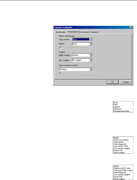
Next, you should specify settings for GLS Weights. You may choose to estimate with no weighting, or with Cross-section weights, Cross-sec- tion SUR, Period weights, Period SUR. The Cross-section SUR setting allows for contemporaneous correlation between cross-sections, while

the Period SUR allows for general correlation of residuals across periods for a specific cross-section. Cross-section weights and Period weights allow for heteroskedasticity in the relevant dimension.

For example, if you select Cross section weights, EViews will estimate a feasible GLS specification assuming the presence of cross-section heteroskedasticity. If you select Cross-sec- tion SUR, EViews estimates a feasible GLS specification correcting for both cross-section heteroskedasticity and contemporaneous correlation. Similarly, Period weights allows for period heteroskedasticity, while Period SUR corrects for both period heteroskedasticity and general correlation of observations within a given cross-section. Note that the SUR specifications are both examples of what is sometimes referred to as the Parks estimator. See the pool discussion of “Generalized Least Squares” on page 864 for additional details.

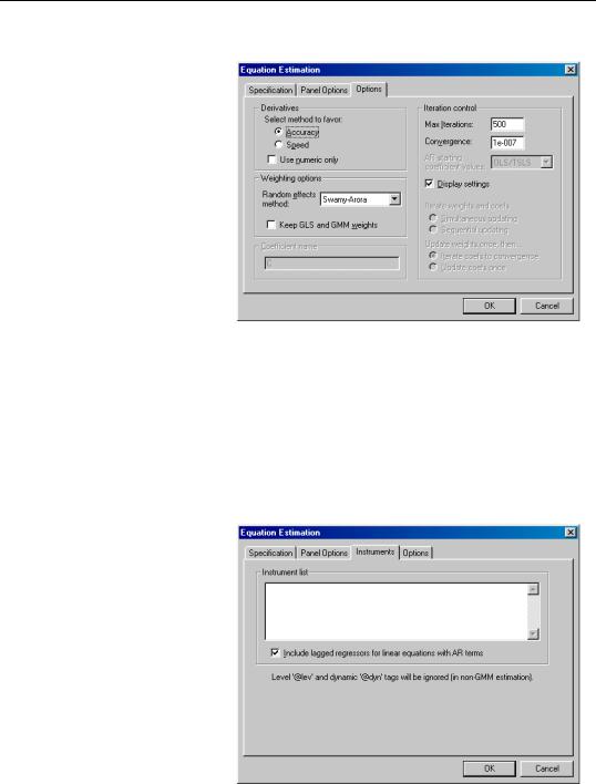
Lastly, you should specify a method for computing coefficient covariances. You may use the combo box labeled Coef covariance method to select from the various robust methods available for computing the coefficient standard errors. The covariance calculations may be chosen to be robust under vari-

ous assumptions, for example, general correlation of observations within a cross-section, or perhaps cross-section heteroskedasticity. Click on the checkbox No d.f. correction to perform the calculations without the leading degree of freedom correction term.

Each of the methods is described in greater detail in “Robust Coefficient Covariances” on page 869 of the pool chapter.

You should note that some combinations of specifications and estimation settings are not currently supported. You may not, for example, estimate random effects models with crosssection specific coefficients, AR terms, or weighting. Furthermore, while two-way random effects specifications are supported for balanced data, they may not be estimated in unbalanced designs.

904—Chapter 29. Panel Estimation

LS Options

Lastly, clicking on the Options tab in the dialog brings up a page displaying computational options for panel estimation. Settings that are not currently applicable will be grayed out.

These options control settings for derivative taking, random effects component variance calculation, coefficient usage, iteration control, and the saving of estimation weights with the equation object.

These options are identical to those found in pool equation estimation, and are described in considerable detail in “Options” on page 849.

Instrumental Variables Estimation

To estimate a pool specification using instrumental variables techniques, you should select

TSLS - Two-Stage Least Squares (and AR) in the Method combo box at the bottom of the main (Specification) dialog page. EViews will respond by creating a four page dialog in which the third page is used to specify your instruments.

While the three original pages are unaffected by this choice of estimation method, note the presence of the new third dialog page labeled Instruments, which you will use to specify your instruments. Click on the Instruments tab to display the new page.

IV Instrument Specification

There are only two parts to the instrumental variables

Estimating a Panel Equation—905

page. First, in the edit box labeled Instrument list, you will list the names of the series or groups of series you wish to use as instruments.

Next, if your specification contains AR terms, you should use the checkbox to indicate whether EViews should automatically create instruments to be used in estimation from lags of the dependent and regressor variables in the original specification. When estimating an equation specified by list that contains AR terms, EViews transforms the linear model and estimates the nonlinear differenced specification. By default, EViews will add lagged values of the dependent and independent regressors to the corresponding lists of instrumental variables to account for the modified specification, but if you wish, you may uncheck this option.

See the pool chapter discussion “Instrumental Variables” on page 867 for additional detail.

GMM Estimation

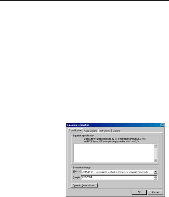
To estimate a panel specification using GMM techniques, you should select GMM / DPD - Generalized Method of Moments / Dynamic Panel Data in the Method combo box at the bottom of the main (Specification) dialog page. Again, you should make certain that your workfile has a panel structure. EViews will respond by displaying a four page dialog that differs significantly from the previous dialogs.

GMM Specification

The specification page is similar to the earlier dialogs. Like the earlier dialogs, you will enter your equation specification in the upper edit box and your sample in the lower edit box.

Note, however, the presence of the Dynamic Panel Wizard... button on the bottom of the dialog. Pressing this button opens a wizard that will aid you in filling out the dialog so that

you may employ dynamic panel data techniques such as the Arellano-Bond 1-step estimator for models with lagged endogenous variables and cross-section fixed effects. We will return to this wizard shortly (“GMM Example” on page 917).

906—Chapter 29. Panel Estimation

GMM Panel Options

Next, click on the Panel Options dialog to specify additional settings for your estimation procedure.

As before, the dialog allows you to indicate the presence of cross-section or period fixed and random effects, to specify GLS weighting, and coefficient covariance calculation methods.

There are, however, notable changes in the available settings.

First, when estimating with GMM, there are two additional choices for handling

cross-section fixed effects. These choices allow you to indicate a transformation method for eliminating the effect from the specification.

You may select Difference to indicate that the estimation procedure should use first differenced data (as in Arellano and Bond, 1991), and you may use Orthogonal Deviations (Arellano and Bover, 1995) to perform an alternative method of removing the individual effects.

Second, the dialog presents you with a new combo box so that you may specify weighting matrices that may provide for additional efficiency of GMM estimation under appropriate assumptions. Here, the available options depend on other settings in the dialog.

In most cases, you may select a method that computes weights under one of the assumptions associated with the robust covariance calculation methods (see “Least Squares Panel Options” on page 902). If you select White cross-section, for example, EViews uses GMM weights that are formed assuming that there is contemporaneous correlation between cross-sections.

If, however, you account for cross-section fixed effects by performing first difference estimation, EViews provides you with a modified set of GMM weights choices. In particular, the Difference (AB 1-step) weights are those associated with the difference transformation. Selecting these weights allows you to estimate the GMM specification typi-

Estimating a Panel Equation—907

cally referred to as Arellano-Bond 1-step estimation. Similarly, you may choose the White period (AB 1-step) weights if you wish to compute Arellano-Bond 2-step or multi-step estimation. Note that the White period weights have been relabeled to indicate that they are typically associated with a specific estimation technique.

Note also that if you estimate your model using difference or orthogonal deviation methods, some GMM weighting methods will no longer be available.

GMM Instruments

Instrument specification in GMM estimation follows the discussion above with a few additional complications.

First, you may enter your instrumental variables as usual by providing the names of series or groups in the edit field. In addition, you may tag instruments as period-specific predetermined instruments, using the “@DYN” keyword, to indicate that the number of implied instruments expands dynamically over time as additional predetermined variables become available.

To specify a set of dynamic instruments associated with the series X, simply enter “@DYN(X)” as an instrument in the list. EViews will, by default, use the series X(-2), X(- 3), ..., X(-T), as instruments for each period (where available). Note that the default set of instruments grows very quickly as the number of periods increases. With 20 periods, for example, there are 171 implicit instruments associated with a single dynamic instrument. To limit the number of implied instruments, you may use only a subset of the instruments by specifying additional arguments to “@DYN” describing a range of lags to be used.

For example, you may limit the maximum number of lags to be used by specifying both a minimum and maximum number of lags as additional arguments. The instrument specification:

@dyn(x, -2, -5)

instructs EViews to include lags of X from 2 to 5 as instruments for each period.

If a single argument is provided, EViews will use it as the minimum number of lags to be considered, and will include all higher ordered lags. For example:

@dyn(x, -5)

includes available lags of X from 5 to the number of periods in the sample.

Second, in specifications estimated using transformations to remove the cross-section fixed effects (first differences or orthogonal deviations), use may use the “@LEV” keyword to instruct EViews to use the instrument in untransformed, or level form. Tagging an instrument with “@LEV” indicates that the instrument is for the transformed equation If

Соседние файлы в папке Docs