

- •Table of Contents
- •What’s New in EViews 5.0
- •What’s New in 5.0
- •Compatibility Notes
- •EViews 5.1 Update Overview
- •Overview of EViews 5.1 New Features
- •Preface
- •Part I. EViews Fundamentals
- •Chapter 1. Introduction
- •What is EViews?
- •Installing and Running EViews
- •Windows Basics
- •The EViews Window
- •Closing EViews
- •Where to Go For Help
- •Chapter 2. A Demonstration
- •Getting Data into EViews
- •Examining the Data
- •Estimating a Regression Model
- •Specification and Hypothesis Tests
- •Modifying the Equation
- •Forecasting from an Estimated Equation
- •Additional Testing
- •Chapter 3. Workfile Basics
- •What is a Workfile?
- •Creating a Workfile
- •The Workfile Window
- •Saving a Workfile
- •Loading a Workfile
- •Multi-page Workfiles
- •Addendum: File Dialog Features
- •Chapter 4. Object Basics
- •What is an Object?
- •Basic Object Operations
- •The Object Window
- •Working with Objects
- •Chapter 5. Basic Data Handling
- •Data Objects
- •Samples
- •Sample Objects
- •Importing Data
- •Exporting Data
- •Frequency Conversion
- •Importing ASCII Text Files
- •Chapter 6. Working with Data
- •Numeric Expressions
- •Series
- •Auto-series
- •Groups
- •Scalars
- •Chapter 7. Working with Data (Advanced)
- •Auto-Updating Series
- •Alpha Series
- •Date Series
- •Value Maps
- •Chapter 8. Series Links
- •Basic Link Concepts
- •Creating a Link
- •Working with Links
- •Chapter 9. Advanced Workfiles
- •Structuring a Workfile
- •Resizing a Workfile
- •Appending to a Workfile
- •Contracting a Workfile
- •Copying from a Workfile
- •Reshaping a Workfile
- •Sorting a Workfile
- •Exporting from a Workfile
- •Chapter 10. EViews Databases
- •Database Overview
- •Database Basics
- •Working with Objects in Databases
- •Database Auto-Series
- •The Database Registry
- •Querying the Database
- •Object Aliases and Illegal Names
- •Maintaining the Database
- •Foreign Format Databases
- •Working with DRIPro Links
- •Part II. Basic Data Analysis
- •Chapter 11. Series
- •Series Views Overview
- •Spreadsheet and Graph Views
- •Descriptive Statistics
- •Tests for Descriptive Stats
- •Distribution Graphs
- •One-Way Tabulation
- •Correlogram
- •Unit Root Test
- •BDS Test
- •Properties
- •Label
- •Series Procs Overview
- •Generate by Equation
- •Resample
- •Seasonal Adjustment
- •Exponential Smoothing
- •Hodrick-Prescott Filter
- •Frequency (Band-Pass) Filter
- •Chapter 12. Groups
- •Group Views Overview
- •Group Members
- •Spreadsheet
- •Dated Data Table
- •Graphs
- •Multiple Graphs
- •Descriptive Statistics
- •Tests of Equality
- •N-Way Tabulation
- •Principal Components
- •Correlations, Covariances, and Correlograms
- •Cross Correlations and Correlograms
- •Cointegration Test
- •Unit Root Test
- •Granger Causality
- •Label
- •Group Procedures Overview
- •Chapter 13. Statistical Graphs from Series and Groups
- •Distribution Graphs of Series
- •Scatter Diagrams with Fit Lines
- •Boxplots
- •Chapter 14. Graphs, Tables, and Text Objects
- •Creating Graphs
- •Modifying Graphs
- •Multiple Graphs
- •Printing Graphs
- •Copying Graphs to the Clipboard
- •Saving Graphs to a File
- •Graph Commands
- •Creating Tables
- •Table Basics
- •Basic Table Customization
- •Customizing Table Cells
- •Copying Tables to the Clipboard
- •Saving Tables to a File
- •Table Commands
- •Text Objects
- •Part III. Basic Single Equation Analysis
- •Chapter 15. Basic Regression
- •Equation Objects
- •Specifying an Equation in EViews
- •Estimating an Equation in EViews
- •Equation Output
- •Working with Equations
- •Estimation Problems
- •Chapter 16. Additional Regression Methods
- •Special Equation Terms
- •Weighted Least Squares
- •Heteroskedasticity and Autocorrelation Consistent Covariances
- •Two-stage Least Squares
- •Nonlinear Least Squares
- •Generalized Method of Moments (GMM)
- •Chapter 17. Time Series Regression
- •Serial Correlation Theory
- •Testing for Serial Correlation
- •Estimating AR Models
- •ARIMA Theory
- •Estimating ARIMA Models
- •ARMA Equation Diagnostics
- •Nonstationary Time Series
- •Unit Root Tests
- •Panel Unit Root Tests
- •Chapter 18. Forecasting from an Equation
- •Forecasting from Equations in EViews
- •An Illustration
- •Forecast Basics
- •Forecasting with ARMA Errors
- •Forecasting from Equations with Expressions
- •Forecasting with Expression and PDL Specifications
- •Chapter 19. Specification and Diagnostic Tests
- •Background
- •Coefficient Tests
- •Residual Tests
- •Specification and Stability Tests
- •Applications
- •Part IV. Advanced Single Equation Analysis
- •Chapter 20. ARCH and GARCH Estimation
- •Basic ARCH Specifications
- •Estimating ARCH Models in EViews
- •Working with ARCH Models
- •Additional ARCH Models
- •Examples
- •Binary Dependent Variable Models
- •Estimating Binary Models in EViews
- •Procedures for Binary Equations
- •Ordered Dependent Variable Models
- •Estimating Ordered Models in EViews
- •Views of Ordered Equations
- •Procedures for Ordered Equations
- •Censored Regression Models
- •Estimating Censored Models in EViews
- •Procedures for Censored Equations
- •Truncated Regression Models
- •Procedures for Truncated Equations
- •Count Models
- •Views of Count Models
- •Procedures for Count Models
- •Demonstrations
- •Technical Notes
- •Chapter 22. The Log Likelihood (LogL) Object
- •Overview
- •Specification
- •Estimation
- •LogL Views
- •LogL Procs
- •Troubleshooting
- •Limitations
- •Examples
- •Part V. Multiple Equation Analysis
- •Chapter 23. System Estimation
- •Background
- •System Estimation Methods
- •How to Create and Specify a System
- •Working With Systems
- •Technical Discussion
- •Vector Autoregressions (VARs)
- •Estimating a VAR in EViews
- •VAR Estimation Output
- •Views and Procs of a VAR
- •Structural (Identified) VARs
- •Cointegration Test
- •Vector Error Correction (VEC) Models
- •A Note on Version Compatibility
- •Chapter 25. State Space Models and the Kalman Filter
- •Background
- •Specifying a State Space Model in EViews
- •Working with the State Space
- •Converting from Version 3 Sspace
- •Technical Discussion
- •Chapter 26. Models
- •Overview
- •An Example Model
- •Building a Model
- •Working with the Model Structure
- •Specifying Scenarios
- •Using Add Factors
- •Solving the Model
- •Working with the Model Data
- •Part VI. Panel and Pooled Data
- •Chapter 27. Pooled Time Series, Cross-Section Data
- •The Pool Workfile
- •The Pool Object
- •Pooled Data
- •Setting up a Pool Workfile
- •Working with Pooled Data
- •Pooled Estimation
- •Chapter 28. Working with Panel Data
- •Structuring a Panel Workfile
- •Panel Workfile Display
- •Panel Workfile Information
- •Working with Panel Data
- •Basic Panel Analysis
- •Chapter 29. Panel Estimation
- •Estimating a Panel Equation
- •Panel Estimation Examples
- •Panel Equation Testing
- •Estimation Background
- •Appendix A. Global Options
- •The Options Menu
- •Print Setup
- •Appendix B. Wildcards
- •Wildcard Expressions
- •Using Wildcard Expressions
- •Source and Destination Patterns
- •Resolving Ambiguities
- •Wildcard versus Pool Identifier
- •Appendix C. Estimation and Solution Options
- •Setting Estimation Options
- •Optimization Algorithms
- •Nonlinear Equation Solution Methods
- •Appendix D. Gradients and Derivatives
- •Gradients
- •Derivatives
- •Appendix E. Information Criteria
- •Definitions
- •Using Information Criteria as a Guide to Model Selection
- •References
- •Index
- •Symbols
- •.DB? files 266
- •.EDB file 262
- •.RTF file 437
- •.WF1 file 62
- •@obsnum
- •Panel
- •@unmaptxt 174
- •~, in backup file name 62, 939
- •Numerics
- •3sls (three-stage least squares) 697, 716
- •Abort key 21
- •ARIMA models 501
- •ASCII
- •file export 115
- •ASCII file
- •See also Unit root tests.
- •Auto-search
- •Auto-series
- •in groups 144
- •Auto-updating series
- •and databases 152
- •Backcast
- •Berndt-Hall-Hall-Hausman (BHHH). See Optimization algorithms.
- •Bias proportion 554
- •fitted index 634
- •Binning option
- •classifications 313, 382
- •Boxplots 409
- •By-group statistics 312, 886, 893
- •coef vector 444
- •Causality
- •Granger's test 389
- •scale factor 649
- •Census X11
- •Census X12 337
- •Chi-square
- •Cholesky factor
- •Classification table
- •Close
- •Coef (coefficient vector)
- •default 444
- •Coefficient
- •Comparison operators
- •Conditional standard deviation
- •graph 610
- •Confidence interval
- •Constant
- •Copy
- •data cut-and-paste 107
- •table to clipboard 437
- •Covariance matrix
- •HAC (Newey-West) 473
- •heteroskedasticity consistent of estimated coefficients 472
- •Create
- •Cross-equation
- •Tukey option 393
- •CUSUM
- •sum of recursive residuals test 589
- •sum of recursive squared residuals test 590
- •Data
- •Database
- •link options 303
- •using auto-updating series with 152
- •Dates
- •Default
- •database 24, 266
- •set directory 71
- •Dependent variable
- •Description
- •Descriptive statistics
- •by group 312
- •group 379
- •individual samples (group) 379
- •Display format
- •Display name
- •Distribution
- •Dummy variables
- •for regression 452
- •lagged dependent variable 495
- •Dynamic forecasting 556
- •Edit
- •See also Unit root tests.
- •Equation
- •create 443
- •store 458
- •Estimation
- •EViews
- •Excel file
- •Excel files
- •Expectation-prediction table
- •Expected dependent variable
- •double 352
- •Export data 114
- •Extreme value
- •binary model 624
- •Fetch
- •File
- •save table to 438
- •Files
- •Fitted index
- •Fitted values
- •Font options
- •Fonts
- •Forecast
- •evaluation 553
- •Foreign data
- •Formula
- •forecast 561
- •Freq
- •DRI database 303
- •F-test
- •for variance equality 321
- •Full information maximum likelihood 698
- •GARCH 601
- •ARCH-M model 603
- •variance factor 668
- •system 716
- •Goodness-of-fit
- •Gradients 963
- •Graph
- •remove elements 423
- •Groups
- •display format 94
- •Groupwise heteroskedasticity 380
- •Help
- •Heteroskedasticity and autocorrelation consistent covariance (HAC) 473
- •History
- •Holt-Winters
- •Hypothesis tests
- •F-test 321
- •Identification
- •Identity
- •Import
- •Import data
- •See also VAR.
- •Index
- •Insert
- •Instruments 474
- •Iteration
- •Iteration option 953
- •in nonlinear least squares 483
- •J-statistic 491
- •J-test 596
- •Kernel
- •bivariate fit 405
- •choice in HAC weighting 704, 718
- •Kernel function
- •Keyboard
- •Kwiatkowski, Phillips, Schmidt, and Shin test 525
- •Label 82
- •Last_update
- •Last_write
- •Latent variable
- •Lead
- •make covariance matrix 643
- •List
- •LM test
- •ARCH 582
- •for binary models 622
- •LOWESS. See also LOESS
- •in ARIMA models 501
- •Mean absolute error 553
- •Metafile
- •Micro TSP
- •recoding 137
- •Models
- •add factors 777, 802
- •solving 804
- •Mouse 18
- •Multicollinearity 460
- •Name
- •Newey-West
- •Nonlinear coefficient restriction
- •Wald test 575
- •weighted two stage 486
- •Normal distribution
- •Numbers
- •chi-square tests 383
- •Object 73
- •Open
- •Option setting
- •Option settings
- •Or operator 98, 133
- •Ordinary residual
- •Panel
- •irregular 214
- •unit root tests 530
- •Paste 83
- •PcGive data 293
- •Polynomial distributed lag
- •Pool
- •Pool (object)
- •PostScript
- •Prediction table
- •Principal components 385
- •Program
- •p-value 569
- •for coefficient t-statistic 450
- •Quiet mode 939
- •RATS data
- •Read 832
- •CUSUM 589
- •Regression
- •Relational operators
- •Remarks
- •database 287
- •Residuals
- •Resize
- •Results
- •RichText Format
- •Robust standard errors
- •Robustness iterations
- •for regression 451
- •with AR specification 500
- •workfile 95
- •Save
- •Seasonal
- •Seasonal graphs 310
- •Select
- •single item 20
- •Serial correlation
- •theory 493
- •Series
- •Smoothing
- •Solve
- •Source
- •Specification test
- •Spreadsheet
- •Standard error
- •Standard error
- •binary models 634
- •Start
- •Starting values
- •Summary statistics
- •for regression variables 451
- •System
- •Table 429
- •font 434
- •Tabulation
- •Template 424
- •Tests. See also Hypothesis tests, Specification test and Goodness of fit.
- •Text file
- •open as workfile 54
- •Type
- •field in database query 282
- •Units
- •Update
- •Valmap
- •find label for value 173
- •find numeric value for label 174
- •Value maps 163
- •estimating 749
- •View
- •Wald test 572
- •nonlinear restriction 575
- •Watson test 323
- •Weighting matrix
- •heteroskedasticity and autocorrelation consistent (HAC) 718
- •kernel options 718
- •White
- •Window
- •Workfile
- •storage defaults 940
- •Write 844
- •XY line
- •Yates' continuity correction 321
|
|
Working with Equations—455 |
|
|
|
|
|
Keywords that return vector or matrix objects |
|||
|
|
|
|
|
@coefcov |
matrix containing the coefficient covariance matrix |
|
|
|
|
|
|
@coefs |
vector of coefficient values |
|
|
|
|
|
|
@stderrs |
vector of standard errors for the coefficients |
|
|
|
|
|
|
@tstats |
vector of t-statistic values for coefficients |
|
|
|
|
|
See also “Equation” (p. 157) in the Command and Programming Reference.
Functions that return a vector or matrix object should be assigned to the corresponding object type. For example, you should assign the results from @tstats to a vector:
vector tstats = eq1.@tstats
and the covariance matrix to a matrix:
matrix mycov = eq1.@cov
You can also access individual elements of these statistics:
scalar pvalue = 1-@cnorm(@abs(eq1.@tstats(4)))
scalar var1 = eq1.@covariance(1,1)
For documentation on using vectors and matrices in EViews, see Chapter 3, “Matrix Language”, on page 23 of the Command and Programming Reference.
Working with Equations
Views of an Equation
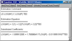
•Representations. Displays the equation in three forms: EViews command form, as an algebraic equation with symbolic coefficients, and as an equation with the estimated values of the coefficients.
You can cut-and-paste from the representations view into any application that supports the Windows clipboard.
•Estimation Output. Displays the equation output results described above.
•Actual, Fitted, Residual. These views display the
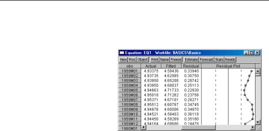
456—Chapter 15. Basic Regression
actual and fitted values of the dependent variable and the residuals from the regression in tabular and graphical form. Actual, Fitted, Residual Table displays these values in table form.
Note that the actual value is always the sum of the fitted value and the residual. Actual, Fitted, Residual Graph displays a standard EViews graph of the actual values, fitted values, and residuals.
Residual Graph plots only the residuals, while the
Standardized Residual
Graph plots the residuals divided by the estimated residual standard deviation.
•ARMA structure.... Provides views which describe the estimated ARMA structure of your residuals. Details on these views are provided in “ARMA Structure” on
page 512.
•Gradients and Derivatives.... Provides views which describe the gradients of the objective function and the information about the computation of any derivatives of the regression function. Details on these views are provided in Appendix D, “Gradients and Derivatives”, on page 963.
•Covariance Matrix. Displays the covariance matrix of the coefficient estimates as a spreadsheet view. To save this covariance matrix as a matrix object, use the @cov function.
•Coefficient Tests, Residual Tests, and Stability Tests. These are views for specification and diagnostic tests and are described in detail in Chapter 19, “Specification and Diagnostic Tests”, beginning on page 569.
Procedures of an Equation
•Specify/Estimate…. Brings up the Equation Specification dialog box so that you can modify your specification. You can edit the equation specification, or change the estimation method or estimation sample.
•Forecast…. Forecasts or fits values using the estimated equation. Forecasting using equations is discussed in Chapter 18, “Forecasting from an Equation”, on page 543.
•Make Residual Series…. Saves the residuals from the regression as a series in the workfile. Depending on the estimation method, you may choose from three types of

Working with Equations—457
residuals: ordinary, standardized, and generalized. For ordinary least squares, only the ordinary residuals may be saved.
•Make Regressor Group. Creates an untitled group comprised of all the variables used in the equation (with the exception of the constant).
•Make Gradient Group. Creates a group containing the gradients of the objective function with respect to the coefficients of the model.
•Make Derivative Group. Creates a group containing the derivatives of the regression function with respect to the coefficients in the regression function.
•Make Model. Creates an untitled model containing a link to the estimated equation. This model can be solved in the usual manner. See Chapter 26, “Models”, on
page 777 for information on how to use models for forecasting and simulations.
•Update Coefs from Equation. Places the estimated coefficients of the equation in the coefficient vector. You can use this procedure to initialize starting values for various estimation procedures.
Residuals from an Equation
The residuals from the default equation are stored in a series object called RESID. RESID may be used directly as if it were a regular series, except in estimation.
RESID will be overwritten whenever you estimate an equation and will contain the residuals from the latest estimated equation. To save the residuals from a particular equation for later analysis, you should save them in a different series so they are not overwritten by the next estimation command. For example, you can copy the residuals into a regular EViews series called RES1 by the command:
series res1 = resid
Even if you have already overwritten the RESID series, you can always create the desired series using EViews’ built-in procedures if you still have the equation object. If your equation is named EQ1, open the equation window and select Proc/Make Residual Series, or enter:
eq1.makeresid res1
to create the desired series.
Regression Statistics
You may refer to various regression statistics through the @-functions described above. For example, to generate a new series equal to FIT plus twice the standard error from the last regression, you can use the command:

458—Chapter 15. Basic Regression
series plus = fit + 2*eq1.@se
To get the t-statistic for the second coefficient from equation EQ1, you could specify
eq1.@tstats(2)
To store the coefficient covariance matrix from EQ1 as a named symmetric matrix, you can use the command:
sym ccov1 = eq1.@cov
See “Keywords that return scalar values” on page 454 for additional details.
Storing and Retrieving an Equation
As with other objects, equations may be stored to disk in data bank or database files. You can also fetch equations from these files.
Equations may also be copied-and-pasted to, or from, workfiles or databases.
EViews even allows you to access equations directly from your databases or another workfile. You can estimate an equation, store it in a database, and then use it to forecast in several workfiles.
See Chapter 4, “Object Basics”, beginning on page 73 and Chapter 10, “EViews Databases”, beginning on page 261 for additional information about objects, databases, and object containers.
Using Estimated Coefficients
The coefficients of an equation are listed in the representations view. By default, EViews will use the C coefficient vector when you specify an equation, but you may explicitly use other coefficient vectors in defining your equation.
These stored coefficients may be used as scalars in generating data. While there are easier ways of generating fitted values (see “Forecasting from an Equation” on page 543), for purposes of illustration, note that we can use the coefficients to form the fitted values from an equation. The command:
series cshat = eq1.c(1) + eq1.c(2)*gdp
forms the fitted value of CS, CSHAT, from the OLS regression coefficients and the independent variables from the equation object EQ1.
Note that while EViews will accept a series generating equation which does not explicitly refer to a named equation:
Working with Equations—459
series cshat = c(1) + c(2)*gdp
and will use the existing values in the C coefficient vector, we strongly recommend that you always use named equations to identify the appropriate coefficients. In general, C will contain the correct coefficient values only immediately following estimation or a coefficient update. Using a named equation, or selecting Proc/Update coefs from equation, guarantees that you are using the correct coefficient values.
An alternative to referring to the coefficient vector is to reference the @coefs elements of your equation (see page 454). For example, the examples above may be written as:
series cshat=eq1.@coefs(1)+eq1.@coefs(2)*gdp
EViews assigns an index to each coefficient in the order that it appears in the representations view. Thus, if you estimate the equation:
equation eq01.ls y=c(10)+b(5)*y(-1)+a(7)*inc
where B and A are also coefficient vectors, then:
•eq01.@coefs(1) contains C(10)
•eq01.@coefs(2) contains B(5)
•eq01.@coefs(3) contains A(7)
This method should prove useful in matching coefficients to standard errors derived from the @stderrs elements of the equation (see Appendix A, “Object, View and Procedure Reference”, on page 153 of the Command and Programming Reference). The @coefs elements allow you to refer to both the coefficients and the standard errors using a common index.
If you have used an alternative named coefficient vector in specifying your equation, you can also access the coefficient vector directly. For example, if you have used a coefficient vector named BETA, you can generate the fitted values by issuing the commands:
equation eq02.ls cs=beta(1)+beta(2)*gdp
series cshat=beta(1)+beta(2)*gdp
where BETA is a coefficient vector. Again, however, we recommend that you use the @coefs elements to refer to the coefficients of EQ02. Alternatively, you can update the coefficients in BETA prior to use by selecting Proc/Update coefs from equation from the equation window. Note that EViews does not allow you to refer to the named equation coefficients EQ02.BETA(1) and EQ02.BETA(2). You must instead use the expressions, EQ02.@COEFS(1) and EQ02.@COEFS(2).