


160—Chapter 7. Working with Data (Advanced)
Auto-series expressions involving alpha series may also evaluate to ordinary series. For example, if NUMER1 is a numeric series and ALPHA1 is an alpha series, you may enter:
show numer1+@len(alpha1)+(alpha1>"cat")
to open a series window containing the results of the operation. Note that the parentheses around the relational comparison are required for correct parsing of the expression.
Date Series
A date series is a standard EViews numeric series that contains valid date values (see “Dates” on page 129 of the Command and Programming Reference). There is nothing that distinguishes a date series from any other numeric series, except for the fact that the values it contains may be interpreted as dates.
Creating a Date Series
There is nothing special about creating a date series. Any method of creating an EViews series may be used to create a numeric series that will be used as a date series.
Displaying a Date Series
The numeric values in a date series are generally of interest only when performing calendar operations. For most purposes, you will wish to see the values of your date series as date strings.
For example, the following series QDATES in our quarterly workfile is a numeric series containing valid date values for the start of each quarter. The numeric values of QDATES depicted here show the number of days since 1 January A.D. 1.
Obviously, this is not the way that most people will wish to view their date series. Accordingly, EViews provides considerable control over the display of the date values in
your series. To change the display, click on the Properties button in the series toolbar, or select View/Properties... from the main menu.
EViews will display a dialog prompting you to change the display properties of the series. While you may change a variety of display settings such as the column width, justification,

Date Series—161
and indentation, here, for the moment, we are more interested in setting the properties of the Numeric Display.
For a date series, there are four settings of interest in the Numeric Display combo box (Period, Day, Day-Time, and Time), with each corresponding to specific information that we wish to display in the series spreadsheet. For example, the Day selection allows you to display date information up to the day in various formats; with year, month, and day all included in the representation.
Let us consider our quarterly workfile example. Here we have selected Period and chosen a specific Date format entry (“YYYY[Q]Q”), which tells EViews that you wish to display the year, followed by the “Q” separator, and then the quarter number. Note also that when Period is selected, there is a Current Workfile setting in the Date format combo box which tells EViews to use the current workfile display settings.
The two checkboxes below the Date for-
mat combo box may be used to modify the selected date format. If you select Two digit year, EViews will only display the last two-digits of the year (if the selected format is “YYYY[Q]Q”, the actual format used will be “YY[Q]Q”); if you select Day/month order, days will precede months in whichever format is selected (if you select “mm/dd/YYYY” as the format for a day display, EViews will use “dd/mm/YYYY”).
Applying this format to the QDATES series, the display changes to show the data in the new format:

162—Chapter 7. Working with Data (Advanced)
If instead we select the Day display, and choose the “YYYY-mm-dd” format, the QDATES spreadsheet will show:
There is one essential fact to remember about the QDATES series. Despite the fact that we have changed the display to show a text representation of the date, QDATES still contains the underlying numeric date values. This is in contrast to using an alpha series to hold a text representation of the date.
If you wish to convert a (numeric) date series into an alpha series, you will need to use the @DATESTR function. If you wish to convert an alpha series into a numeric date series, you will need to use the @DATEVAL function. See “Translating between Date Strings and Date Numbers” on page 135 of the Command and Programming Reference for details.

Value Maps—163
Editing a Date Series
You may edit a date series either by either date numbers, or if the series is displayed using a date format, by entering date strings directly.
Suppose, for example, that we have our date series from above and that we wish to change a value. If we are displaying the series with date formatting, we may enter a date string, which EViews will automatically convert into a date number.
For example, we may edit our QDATES series by entering a valid date string (“April 10, 1992”), which EViews will convert into a date number (727297.0), and then display as a
date string (“1992-04-10”). See “Free-format Conversion” on page 137 of the Command and Programming Reference for details on automatic translation of strings to date values.
Note, however, that if we were to enter the same string value in the series when the display is set to show numeric values, EViews will not attempt to interpret the string and will enter an NA in the series.
Value Maps
You may use the valmap object to create a value map (or map, for short) that assigns descriptive labels to values in numeric or alpha series. The practice of mapping observation values to labels allows you to hold your data in encoded or abbreviated form, while displaying the results using easy-to-interpret labels.

164—Chapter 7. Working with Data (Advanced)
Perhaps the most common example of encoded data occurs when you have categorical identifiers that are given by integer values. For example, we may have a numeric series FEMALE containing a binary indicator for whether an individual is a female (1) or a male (0).
Numeric encodings of this type are commonly employed, since they allow one to work with the numeric values of FEMALE. One may, for example, compute the mean
value of the FEMALE variable, which will provide the proportion of observations that are female.
On the other hand, numeric encoding of categorical data has the disadvantage that one must always translate from the numeric values to the underlying categorical data types. For example, a one-way tabulation of the FEMALE data produces the output:
Tabulation of FEMALE |
|
|
|
|
Date: 09/30/03 |
Time: 11:36 |
|
|
|
Sample: 1 6 |
|
|
|
|
Included observations: 6 |
|
|
|
|
Number of categories: 2 |
|
|
|
|
|
|
|
|
|
|
|
|
|
|
|
|
|
Cumulative |
Cumulative |
Value |
Count |
Percent |
Count |
Percent |
0 |
3 |
50.00 |
3 |
50.00 |
1 |
3 |
50.00 |
6 |
100.00 |
Total |
6 |
100.00 |
6 |
100.00 |
|
|
|
|
|
|
|
|
|
|
Interpretation of this output requires that the viewer remember that the FEMALE series is encoded so that the “0” value represents “Male” and the “1” represents “Female”. The example above would be easier to interpret if the first column showed the text representations of the categories in place of the numeric values.
Valmaps allow us to combine the benefits of descriptive text data values with the ease of working with a numeric encoding of the data. In cases where we define value maps for alphanumeric data, the associations allow us to use space saving abbreviations for the underlying data along with more descriptive labels to be used in presenting output.

Value Maps—165
Defining a Valmap
To create a valmap object, select
Object/New Object.../ValMap from the main menu and optionally enter an object name, or enter the keyword “VALMAP” in the command line, followed by an optional name. EViews will open a valmap object.
You will enter your new mappings below the double line by typing or by copy-and-pasting. In the Value column,
you should enter the values for which you wish to provide labels; in the Label column, you will enter the corresponding text label. Here, we define a valmap named FEMALEMAP in which the value 0 is mapped to the string “Male”, and the value 1 is mapped to the string “Female”.
The two special entries above the double line should be used to define mappings for blank strings and numeric missing values. The default mapping is to represent blank strings as themselves, and to represent numeric missing values with the text “NA”. You may change these defaults by entering the appropriate text in the Label column. For example, to change the representation of missing numeric values to, say, a period, simply type the “.” character in the appropriate cell.
We caution that when working with maps, EViews will look for exact equality between the value in a series and the value in the valmap. Such an equality comparison is subject to the usual issues associated with comparing floating point numbers. To mitigate these issues and to facilitate mapping large numbers of values, EViews allows you to define value maps using intervals.
To map an interval, simply enter a range of values in the Value column and the associated label in the Label column. You may use round and square parentheses, to denote open (“(“, “)“) or closed (“[“, “]”) interval endpoints, and the special values “–INF” and “INF” to represent minus and plus infinity.
Using interval mapping, we require only
three entries to map all of the negative values to the string “negative”, the positive values to the string “positive”, and the value 0 to the string “zero”. Note that the first interval in

166—Chapter 7. Working with Data (Advanced)
our example, “[–inf, 0)”, is mathematically incorrect since the lower bound is not closed, but EViews allows the closed interval syntax in this case since there is no possibility of confusion.
While the primary use for valmaps will be to map numeric series values, there is nothing stopping you from defining labels corresponding to alpha series values (note that value and label matching is case sensitive). One important application of string value mapping is to expand abbreviations. For example, one might wish to map the U.S. Postal Service state abbreviations to full state names.
Since valmaps may be used with both
numeric and alpha series, the text entries in the Value column may generally be used to match both numeric and alphanumeric values. For example, if you enter the text “0” as your value, EViews treats the entry as representing either a numeric 0 or the string value “0”. Similarly, entering the text string “[0,1]” will match both numeric values in the interval, as well as the string value “[0,1]”.
There is one exception to this dual interpretation. You may, in the process of defining a given valmap, provide an entry that conflicts with a previous entry. EViews will automatically identify the conflict, and will convert the latter entry into a string-only valmap entry.
For example, if the first line of your valmap maps 0 to “Zero”, a line that maps 0 to “New Zero”, or one that maps “[0,
1]” to “Unit interval” conflicts with the existing entry. In the latter cases, the conflicting maps will be treated as text maps. Such a map is identified by enclosing the entry with quotation marks. Here, EViews has automatically added the enclosing quotation marks to indicate that the latter two label entries will only be interpreted as string maps, and not as numeric maps.
Once you have defined your mappings, click on the Update button on the toolbar to validate the object. EViews will examine your valmap and will remove entries with values that

Value Maps—167
are exact duplicates. In this example, the last entry, which maps the string “0” to the value “New Zero” will be removed since it conflicts with the first line. The second entry will be retained since it is not an exact duplicate of any other entry. It will, however, be interpreted only as a string since the numeric interpretation would lead to multiple mappings for the value 0.
Assigning a Valmap to a Series
To use a valmap, you need to instruct EViews to display the values of the map in place of the underlying data. Before working with a valmap, you should be certain that you have updated and validated your valmap by pressing the Update button on the valmap toolbar.
First, you must assign the value map to your series by modifying the series properties. Open the series window and select
View/Properties... or click on the Properties button in the series toolbar to open the properties dialog. Click on the Value Map tab to display the value map name edit field.
If the edit field is blank, a value map has not been associated with this series. To assign a valmap, simply enter the name of a valmap object in the edit field and click on OK.
EViews will validate the entry and apply the specified map to the series. Note that to be valid, the valmap must exist in the same workfile page as the series to which it is assigned.
Using the Valmap Tools
EViews provides a small set of object-specific views and procedures that will aid you in working with valmaps.
Sorting Valmap Entries
You may add your valmap entries in any order without changing the behavior of the map. However, when viewing the contents of the map, you may find it useful to see the entries in sorted order.
168—Chapter 7. Working with Data (Advanced)
To sort the contents of your map, click on Proc/Sort...
from the main valmap menu. EViews provides you with the choice of sorting by the value column using numeric order (Value - Numeric), sorting by the value column using text order (Value - Text) or sorting by the label column (Label).
In the first two cases, we sort by the values in the first
column of the valmap. The difference between the choices is apparent when you note that the ordering of the entries “9” and “10” depends upon whether we are interpreting the sort as a numeric sort, or as a text sort. Selecting Value - Numeric tells EViews that where possible, you wish to interpret strings as numbers when performing comparisons (so that “9” is less than “10”); selecting Value - Text says that all values should be treated as text for purposes of comparison (so that “10” is less than “9”).
Click on OK to accept the sort settings.
Examining Properties of a Valmap
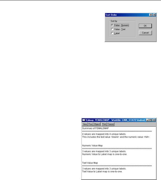
You may examine a summary of your valmap by selecting View/Statistics in the valmap window. EViews will display a view showing the properties of the labels defined in the object.
The top portion of the view shows the number of mappings in the valmap, and the number of unique labels used in those definitions. Here we see that the valmap has four definitions, which map four values into four unique labels. Two of the four definitions are the special entries for blank strings and the numeric NA value.
The remaining portions of the view provide a detailed summary of the valmap describing the properties of the map when applied to numeric and to text values.
When applied to an ordinary numeric series, our FEMALEMAP example contains three relevant definitions that provide labels for the values 0, 1, and NA. Here, EViews reports that the numeric value mapping is one-to-one since there are no two values that produce the same value label.
Value Maps—169
The output also reports that the FEMALEMAP has three relevant definitions for mapping the three text values, “0”, “1”, and the blank string, into three unique labels. We see that the text interpreted maps are also one-to-one.
Note that in settings where we map an interval into a given label, or where a given text label is repeated for multiple values, EViews will report a many-to-one mapping. Knowing that a valmap is many-to-one is important since it implies that the values of the underlying source series are not uniquely identified by the label values. This lack of identification has important implications in editing mapped series and in interpreting the results from various statistical output (see “Editing a Mapped Series” on page 171 and “Valmap Definition Cautions” on page 175).
Tracking Valmap Usage
A single valmap may be applied to more than one series. You may track the usage of a given valmap by selecting View/Usage from the valmap main menu. EViews will examine every numeric and alpha series in the workfile page to determine which, if any, have applied the specified valmap.
The valmap view then changes to show the number and names of the series that employ the valmap, with separate lists for the numeric and the alpha series. Here we see that there is a single numeric series named FEMALE that uses FEMALEMAP.
Working with a Mapped Series
Once you assign a map to a series, EViews allows you to display and edit your series
using the mapped values and will use the labels when displaying the output from selected procedures.
Displaying series values
By default, once you apply a value map to a series, the EViews spreadsheet view will change to display the newly mapped values.

170—Chapter 7. Working with Data (Advanced)
For example, after applying the FEMALEMAP to our FEMALE series, the series spreadsheet view changes to show the labels associated with each value instead of the underlying encoded values. Note that the display format combo box usually visible in series toolbar indicates that EViews is displaying the Default series values, so that it shows the labels “Male” and “Female” rather than the underlying 0 and 1 values.
Note that if any of the values in the series does not have a corresponding valmap entry, EViews will display a mix of labeled and unlabeled values, with the unlabeled value “showing through” the mapping. For example, if the last observation in the FEMALE series had the value 3, the series spreadsheet will show observations with “Male” and “Female” corresponding to the mapped values, as well as the unmapped value 3.
There may be times when you wish to view the underlying series values instead of the labels. There are two possible approaches. First, you may remove the valmap assignment from the series. Simply go to the Properties dialog, and delete the name of the valmap object from the Value Map page. The display will revert to showing the underlying values. Less drastically, you may use the display method combo box to change the display format for the spreadsheet view.
If you select Raw Data, the series spreadsheet view will change to show the underlying series data.

Value Maps—171
Editing a Mapped Series
To edit the values of your mapped series, first make certain you are in edit mode, then enter the desired values, either by typing in the edit field, or by pasting from the clipboard. How EViews interprets your input will differ depending upon the current display format for the series.
If your mapped series is displayed in its original form using the Raw Data setting, EViews will interpret any input as representing the underlying series values, and will place the input directly into the series. For example, if our FEMALE series is displayed using the Raw Data setting, any numeric input will be entered directly in the series, and any string input will be interpreted as an NA value.
In contrast, if the series is displayed using the Default setting, EViews will use the attached valmap both in displaying the labeled values and in interpreting any input. In this setting, EViews will first examine the attached valmap to determine whether the given input value is also a label in the valmap. If a matching entry is found, and the label matches a unique underlying value, EViews will put the value in the series. If there is no matching valmap label entry, or if there is an entry but the corresponding value is ambiguous, EViews will put the input value directly into the series. One implication of this behavior is that so long as the underlying values are not themselves valmap labels, you may enter data in either mapped or unmapped form. Note, again, that text value and label matching is case-sensi- tive.
Let us consider a simple example.
Suppose that the FEMALE series is set to display mapped values, and that you enter the value “Female”. EViews will examine the assigned valmap, determine that “Female” corresponds to the valmap value “1”, and then assign this value to the series. Since “1” is a valid form of numeric input, the value 1 will be placed in the series. Note that even though we have
entered 1 into the series, the mapped spreadsheet view will continue to show the value “Female”.
Alternatively, we could have entered a “1” corresponding to the underlying numeric value. Since “1” is not a valmap label, EViews will put the value 1 in the series, which will be displayed using the label “Female”.

172—Chapter 7. Working with Data (Advanced)
While quite useful, entering data in mapped display mode requires some care, as your results may be somewhat unexpected. For one, you should bear in mind that the required reverse lookup of values associated with a given input requires an exact match of the input to a label value, and a one-to-one correspondence between the given label and a valmap value. If this condition is not met, the original input value will be placed in the series.
Consider, for example, the result of entering the string “female” instead of “Female”. In this case, there is no matching valmap label entry, so EViews will put the input value, “female”, into the series. Since FEMALE is a numeric series, the resulting value will be an NA, and the display will show the mapped value for numeric missing values.
Similarly, suppose you enter “3” into the last observation of the FEMALE series. Again, EViews does not find a corresponding valmap label entry, so the input is entered directly into the series. In this case, the input represents a valid number so that the resulting value will be a 3. Since there is no valmap entry for this value, the underlying value will be displayed.
Lastly, note that if the matching valmap label corresponds to multiple underlying values, EViews will be unable to perform the reverse lookup. If, for example, we modify our valmap so that the interval “[1, 10]” (instead of just the value 1) maps to the label “Female”, then when you enter “Female” as your input, it is impossible to determine a unique value for the series. In this case, EViews will enter the original input, “Female”, directly into the series, resulting in an NA value.
See “Valmap Definition Cautions” on page 175 for additional cautionary notes.
Using a Mapped Series
You may use a mapped series as though it were any series. We emphasize the fact that the mapped values of a series are not replacements of the underlying data; they are only labels to be used in output. Thus, when performing numeric calculations with a series, EViews will always use the underlying values of the series, not the label values. For example, if you map the numeric value -99 to the text “NA”, and take the absolute value of the mapped numeric series containing that value, you will get the value 99, and not a missing value.
In appropriate settings (where the series values are treated as categories), EViews routines will use the labels when displaying output. For example, a one-way frequency tabulation of the FEMALE series with the assigned FEMALEMAP yields:

Value Maps—173
Tabulation of FEMALE
Date: 10/01/03 Time: 09:27
Sample: 1 6
Included observations: 6
Number of categories: 2
|
|
|
Cumulative |
Cumulative |
Value |
Count |
Percent |
Count |
Percent |
Male |
3 |
50.00 |
3 |
50.00 |
Female |
3 |
50.00 |
6 |
100.00 |
Total |
6 |
100.00 |
6 |
100.00 |
|
|
|
|
|
|
|
|
|
|
Similarly, when computing descriptive statistics for the SALES data categorized by the values of the FEMALE series, we have:
Descriptive Statistics for SALES
Categorized by values of FEMALE
Date: 10/01/03 Time: 09:30
Sample: 1 6
Included observations: 6
FEMALE |
Mean |
Std. Dev. |
Obs. |
Male |
323.3333 |
166.2328 |
3 |
Female |
263.3333 |
169.2139 |
3 |
All |
293.3333 |
153.5795 |
6 |
|
|
|
|
|
|
|
|
Valmap Functions
To facilitate working with valmaps, three new genr functions are provided which allow you to translate between unmapped and mapped values. These functions may be used as part of standard series or alpha expressions.
First, to obtain the mapped values corresponding to a set of numbers or strings, you may use the command:
@MAP(arg[, map_name])
where arg is a numeric or string series expression or literal, and the optional map_name is the name of a valmap object. If map_name is not provided, EViews will attempt to determine the map by inspecting arg. This attempt will succeed only if arg is a numeric series or alpha series that has previously been mapped.
Let us consider our original example where the FEMALEMAP maps 0 to “Male” and 1 to “Female”. Suppose that we have two series that contain the values 0 and 1. The first series,

174—Chapter 7. Working with Data (Advanced)
MAPPEDSER, has previously applied the FEMALEMAP, while the latter series, UNMAPPEDSER, has not.
Then the commands:
alpha s1 = @map(mappedser)
alpha s2 = @map(mappedser, femalemap)
are equivalent. Both return the labels associated with the numeric values in the series. The first command uses the assigned valmap to determine the mapped values, while the second uses FEMALEMAP explicitly.
Alternately, the command:
alpha s3 = @map(unmappedser)
will generate an error since there is no valmap assigned to the series. To use @MAP in this context, you must provide the name of a valmap, as in:
alpha s4 = @map(unmappedser, femalemap)
which will return the mapped values of UNMAPPEDSER, using the valmap FEMALEMAP.
Conversely, you may obtain the numeric values associated with a set of string value labels using the @UNMAP function. The @UNMAP function takes the general form:
@UNMAP(arg, map_name)
to return the numeric values that have been mapped into the string given in the string expression or literal arg, where map_name is the name of a valmap object. Note that if a given label is associated with multiple numeric values, the missing value NA will be returned. Note that the map_name argument is required with the @UNMAP function.
Suppose, for example, that you have an alpha series STATEAB that contains state abbreviations (“AK”, “AL”, etc.) and a valmap STATEMAP that maps numbers to the abbreviations. Then:
series statecode = @unmap(stateab, statemap)
will contain the numeric values associated with each value of STATEAB.
Similarly, you may obtain the string values associated with a set of string value labels using:
@UNMAPTXT(arg, map_name)
where arg is a string expression or literal, and map_name is the name of a valmap object. @UNMAPTXT will return the underlying string values that are mapped into the string labels provided in arg. If a given label is associated with multiple values, the missing blank string “” will be returned.

Value Maps—175
Valmap Definition Cautions
EViews allows you to define quite general value maps that may be used with both numeric and alpha series. While potentially useful, the generality comes with a cost, since if used carelessly, valmaps can cause confusion. Accordingly, we caution you that there are many features of valmaps that should be used with care. To illustrate the issues, we list a few of the more problematic cases.
Many-to-one Valmaps
A many-to-one valmap is a useful tool for creating labels that divide series values into broad categories. For example, you may assign the label “High” to a range of values, and the label “Low” to a different range of values so that you may, when displaying the series labels, easily view the classification of an observation.
The downside to many-to-one valmaps is that they make interpreting some types of output considerably more difficult. Suppose, for example, that we construct a valmap in which several values are mapped to the label “Female”. If we then display a one-way frequency table for a series that uses the valmap, the label “Female” may appear as multiple entries. Such a table is almost impossible to interpret since there is no way to distinguish between the various “Female” values.
A series with an attached many-to-one valmap is also more difficult to edit when viewing labels since EViews may be unable to identify a unique value corresponding to a given label. In these cases, EViews will assign a missing value to the series, which may lead to confusion (see “Editing a Mapped Series” on page 171).
Mapping Label Values
Defining a map in which one of the label values is itself a value that is mapped to a label can cause confusion. Suppose, for example, that we have a valmap with two entries: the first maps the value 6 to the label “six”, and the second maps the value “six” to the label “high”.
Now consider editing an alpha series that has this valmap attached. If we use the Default display, EViews will show the labeled values. Thus, the underlying value “six” will display as the value “high”; while the value “6” will display as “six”. Since the string “six” is used both as a label and as a value, in this setting we have the odd result that it must be entered indirectly. Thus, to enter the string “six” in the alpha series, we have the counterintuitive result that you must type “high” instead of “six”, since entering the latter value will put “6” in the series.
Note, however, that if you display the series in Raw Data form, all data entry is direct; entering “six” will put the value “six” into the series and entering “high” will put the value “high” in the series.

176—Chapter 7. Working with Data (Advanced)
Mapping Values to Numbers
Along the same lines, we strongly recommend that you not define value maps in which numeric values can be mapped to labels that appear to be numeric values. Electing, for example, to define a valmap where the value 5 is mapped to the label “6” and the value 6 is mapped to the label “5”, is bound to lead to confusion.