

- •Table of Contents
- •What’s New in EViews 5.0
- •What’s New in 5.0
- •Compatibility Notes
- •EViews 5.1 Update Overview
- •Overview of EViews 5.1 New Features
- •Preface
- •Part I. EViews Fundamentals
- •Chapter 1. Introduction
- •What is EViews?
- •Installing and Running EViews
- •Windows Basics
- •The EViews Window
- •Closing EViews
- •Where to Go For Help
- •Chapter 2. A Demonstration
- •Getting Data into EViews
- •Examining the Data
- •Estimating a Regression Model
- •Specification and Hypothesis Tests
- •Modifying the Equation
- •Forecasting from an Estimated Equation
- •Additional Testing
- •Chapter 3. Workfile Basics
- •What is a Workfile?
- •Creating a Workfile
- •The Workfile Window
- •Saving a Workfile
- •Loading a Workfile
- •Multi-page Workfiles
- •Addendum: File Dialog Features
- •Chapter 4. Object Basics
- •What is an Object?
- •Basic Object Operations
- •The Object Window
- •Working with Objects
- •Chapter 5. Basic Data Handling
- •Data Objects
- •Samples
- •Sample Objects
- •Importing Data
- •Exporting Data
- •Frequency Conversion
- •Importing ASCII Text Files
- •Chapter 6. Working with Data
- •Numeric Expressions
- •Series
- •Auto-series
- •Groups
- •Scalars
- •Chapter 7. Working with Data (Advanced)
- •Auto-Updating Series
- •Alpha Series
- •Date Series
- •Value Maps
- •Chapter 8. Series Links
- •Basic Link Concepts
- •Creating a Link
- •Working with Links
- •Chapter 9. Advanced Workfiles
- •Structuring a Workfile
- •Resizing a Workfile
- •Appending to a Workfile
- •Contracting a Workfile
- •Copying from a Workfile
- •Reshaping a Workfile
- •Sorting a Workfile
- •Exporting from a Workfile
- •Chapter 10. EViews Databases
- •Database Overview
- •Database Basics
- •Working with Objects in Databases
- •Database Auto-Series
- •The Database Registry
- •Querying the Database
- •Object Aliases and Illegal Names
- •Maintaining the Database
- •Foreign Format Databases
- •Working with DRIPro Links
- •Part II. Basic Data Analysis
- •Chapter 11. Series
- •Series Views Overview
- •Spreadsheet and Graph Views
- •Descriptive Statistics
- •Tests for Descriptive Stats
- •Distribution Graphs
- •One-Way Tabulation
- •Correlogram
- •Unit Root Test
- •BDS Test
- •Properties
- •Label
- •Series Procs Overview
- •Generate by Equation
- •Resample
- •Seasonal Adjustment
- •Exponential Smoothing
- •Hodrick-Prescott Filter
- •Frequency (Band-Pass) Filter
- •Chapter 12. Groups
- •Group Views Overview
- •Group Members
- •Spreadsheet
- •Dated Data Table
- •Graphs
- •Multiple Graphs
- •Descriptive Statistics
- •Tests of Equality
- •N-Way Tabulation
- •Principal Components
- •Correlations, Covariances, and Correlograms
- •Cross Correlations and Correlograms
- •Cointegration Test
- •Unit Root Test
- •Granger Causality
- •Label
- •Group Procedures Overview
- •Chapter 13. Statistical Graphs from Series and Groups
- •Distribution Graphs of Series
- •Scatter Diagrams with Fit Lines
- •Boxplots
- •Chapter 14. Graphs, Tables, and Text Objects
- •Creating Graphs
- •Modifying Graphs
- •Multiple Graphs
- •Printing Graphs
- •Copying Graphs to the Clipboard
- •Saving Graphs to a File
- •Graph Commands
- •Creating Tables
- •Table Basics
- •Basic Table Customization
- •Customizing Table Cells
- •Copying Tables to the Clipboard
- •Saving Tables to a File
- •Table Commands
- •Text Objects
- •Part III. Basic Single Equation Analysis
- •Chapter 15. Basic Regression
- •Equation Objects
- •Specifying an Equation in EViews
- •Estimating an Equation in EViews
- •Equation Output
- •Working with Equations
- •Estimation Problems
- •Chapter 16. Additional Regression Methods
- •Special Equation Terms
- •Weighted Least Squares
- •Heteroskedasticity and Autocorrelation Consistent Covariances
- •Two-stage Least Squares
- •Nonlinear Least Squares
- •Generalized Method of Moments (GMM)
- •Chapter 17. Time Series Regression
- •Serial Correlation Theory
- •Testing for Serial Correlation
- •Estimating AR Models
- •ARIMA Theory
- •Estimating ARIMA Models
- •ARMA Equation Diagnostics
- •Nonstationary Time Series
- •Unit Root Tests
- •Panel Unit Root Tests
- •Chapter 18. Forecasting from an Equation
- •Forecasting from Equations in EViews
- •An Illustration
- •Forecast Basics
- •Forecasting with ARMA Errors
- •Forecasting from Equations with Expressions
- •Forecasting with Expression and PDL Specifications
- •Chapter 19. Specification and Diagnostic Tests
- •Background
- •Coefficient Tests
- •Residual Tests
- •Specification and Stability Tests
- •Applications
- •Part IV. Advanced Single Equation Analysis
- •Chapter 20. ARCH and GARCH Estimation
- •Basic ARCH Specifications
- •Estimating ARCH Models in EViews
- •Working with ARCH Models
- •Additional ARCH Models
- •Examples
- •Binary Dependent Variable Models
- •Estimating Binary Models in EViews
- •Procedures for Binary Equations
- •Ordered Dependent Variable Models
- •Estimating Ordered Models in EViews
- •Views of Ordered Equations
- •Procedures for Ordered Equations
- •Censored Regression Models
- •Estimating Censored Models in EViews
- •Procedures for Censored Equations
- •Truncated Regression Models
- •Procedures for Truncated Equations
- •Count Models
- •Views of Count Models
- •Procedures for Count Models
- •Demonstrations
- •Technical Notes
- •Chapter 22. The Log Likelihood (LogL) Object
- •Overview
- •Specification
- •Estimation
- •LogL Views
- •LogL Procs
- •Troubleshooting
- •Limitations
- •Examples
- •Part V. Multiple Equation Analysis
- •Chapter 23. System Estimation
- •Background
- •System Estimation Methods
- •How to Create and Specify a System
- •Working With Systems
- •Technical Discussion
- •Vector Autoregressions (VARs)
- •Estimating a VAR in EViews
- •VAR Estimation Output
- •Views and Procs of a VAR
- •Structural (Identified) VARs
- •Cointegration Test
- •Vector Error Correction (VEC) Models
- •A Note on Version Compatibility
- •Chapter 25. State Space Models and the Kalman Filter
- •Background
- •Specifying a State Space Model in EViews
- •Working with the State Space
- •Converting from Version 3 Sspace
- •Technical Discussion
- •Chapter 26. Models
- •Overview
- •An Example Model
- •Building a Model
- •Working with the Model Structure
- •Specifying Scenarios
- •Using Add Factors
- •Solving the Model
- •Working with the Model Data
- •Part VI. Panel and Pooled Data
- •Chapter 27. Pooled Time Series, Cross-Section Data
- •The Pool Workfile
- •The Pool Object
- •Pooled Data
- •Setting up a Pool Workfile
- •Working with Pooled Data
- •Pooled Estimation
- •Chapter 28. Working with Panel Data
- •Structuring a Panel Workfile
- •Panel Workfile Display
- •Panel Workfile Information
- •Working with Panel Data
- •Basic Panel Analysis
- •Chapter 29. Panel Estimation
- •Estimating a Panel Equation
- •Panel Estimation Examples
- •Panel Equation Testing
- •Estimation Background
- •Appendix A. Global Options
- •The Options Menu
- •Print Setup
- •Appendix B. Wildcards
- •Wildcard Expressions
- •Using Wildcard Expressions
- •Source and Destination Patterns
- •Resolving Ambiguities
- •Wildcard versus Pool Identifier
- •Appendix C. Estimation and Solution Options
- •Setting Estimation Options
- •Optimization Algorithms
- •Nonlinear Equation Solution Methods
- •Appendix D. Gradients and Derivatives
- •Gradients
- •Derivatives
- •Appendix E. Information Criteria
- •Definitions
- •Using Information Criteria as a Guide to Model Selection
- •References
- •Index
- •Symbols
- •.DB? files 266
- •.EDB file 262
- •.RTF file 437
- •.WF1 file 62
- •@obsnum
- •Panel
- •@unmaptxt 174
- •~, in backup file name 62, 939
- •Numerics
- •3sls (three-stage least squares) 697, 716
- •Abort key 21
- •ARIMA models 501
- •ASCII
- •file export 115
- •ASCII file
- •See also Unit root tests.
- •Auto-search
- •Auto-series
- •in groups 144
- •Auto-updating series
- •and databases 152
- •Backcast
- •Berndt-Hall-Hall-Hausman (BHHH). See Optimization algorithms.
- •Bias proportion 554
- •fitted index 634
- •Binning option
- •classifications 313, 382
- •Boxplots 409
- •By-group statistics 312, 886, 893
- •coef vector 444
- •Causality
- •Granger's test 389
- •scale factor 649
- •Census X11
- •Census X12 337
- •Chi-square
- •Cholesky factor
- •Classification table
- •Close
- •Coef (coefficient vector)
- •default 444
- •Coefficient
- •Comparison operators
- •Conditional standard deviation
- •graph 610
- •Confidence interval
- •Constant
- •Copy
- •data cut-and-paste 107
- •table to clipboard 437
- •Covariance matrix
- •HAC (Newey-West) 473
- •heteroskedasticity consistent of estimated coefficients 472
- •Create
- •Cross-equation
- •Tukey option 393
- •CUSUM
- •sum of recursive residuals test 589
- •sum of recursive squared residuals test 590
- •Data
- •Database
- •link options 303
- •using auto-updating series with 152
- •Dates
- •Default
- •database 24, 266
- •set directory 71
- •Dependent variable
- •Description
- •Descriptive statistics
- •by group 312
- •group 379
- •individual samples (group) 379
- •Display format
- •Display name
- •Distribution
- •Dummy variables
- •for regression 452
- •lagged dependent variable 495
- •Dynamic forecasting 556
- •Edit
- •See also Unit root tests.
- •Equation
- •create 443
- •store 458
- •Estimation
- •EViews
- •Excel file
- •Excel files
- •Expectation-prediction table
- •Expected dependent variable
- •double 352
- •Export data 114
- •Extreme value
- •binary model 624
- •Fetch
- •File
- •save table to 438
- •Files
- •Fitted index
- •Fitted values
- •Font options
- •Fonts
- •Forecast
- •evaluation 553
- •Foreign data
- •Formula
- •forecast 561
- •Freq
- •DRI database 303
- •F-test
- •for variance equality 321
- •Full information maximum likelihood 698
- •GARCH 601
- •ARCH-M model 603
- •variance factor 668
- •system 716
- •Goodness-of-fit
- •Gradients 963
- •Graph
- •remove elements 423
- •Groups
- •display format 94
- •Groupwise heteroskedasticity 380
- •Help
- •Heteroskedasticity and autocorrelation consistent covariance (HAC) 473
- •History
- •Holt-Winters
- •Hypothesis tests
- •F-test 321
- •Identification
- •Identity
- •Import
- •Import data
- •See also VAR.
- •Index
- •Insert
- •Instruments 474
- •Iteration
- •Iteration option 953
- •in nonlinear least squares 483
- •J-statistic 491
- •J-test 596
- •Kernel
- •bivariate fit 405
- •choice in HAC weighting 704, 718
- •Kernel function
- •Keyboard
- •Kwiatkowski, Phillips, Schmidt, and Shin test 525
- •Label 82
- •Last_update
- •Last_write
- •Latent variable
- •Lead
- •make covariance matrix 643
- •List
- •LM test
- •ARCH 582
- •for binary models 622
- •LOWESS. See also LOESS
- •in ARIMA models 501
- •Mean absolute error 553
- •Metafile
- •Micro TSP
- •recoding 137
- •Models
- •add factors 777, 802
- •solving 804
- •Mouse 18
- •Multicollinearity 460
- •Name
- •Newey-West
- •Nonlinear coefficient restriction
- •Wald test 575
- •weighted two stage 486
- •Normal distribution
- •Numbers
- •chi-square tests 383
- •Object 73
- •Open
- •Option setting
- •Option settings
- •Or operator 98, 133
- •Ordinary residual
- •Panel
- •irregular 214
- •unit root tests 530
- •Paste 83
- •PcGive data 293
- •Polynomial distributed lag
- •Pool
- •Pool (object)
- •PostScript
- •Prediction table
- •Principal components 385
- •Program
- •p-value 569
- •for coefficient t-statistic 450
- •Quiet mode 939
- •RATS data
- •Read 832
- •CUSUM 589
- •Regression
- •Relational operators
- •Remarks
- •database 287
- •Residuals
- •Resize
- •Results
- •RichText Format
- •Robust standard errors
- •Robustness iterations
- •for regression 451
- •with AR specification 500
- •workfile 95
- •Save
- •Seasonal
- •Seasonal graphs 310
- •Select
- •single item 20
- •Serial correlation
- •theory 493
- •Series
- •Smoothing
- •Solve
- •Source
- •Specification test
- •Spreadsheet
- •Standard error
- •Standard error
- •binary models 634
- •Start
- •Starting values
- •Summary statistics
- •for regression variables 451
- •System
- •Table 429
- •font 434
- •Tabulation
- •Template 424
- •Tests. See also Hypothesis tests, Specification test and Goodness of fit.
- •Text file
- •open as workfile 54
- •Type
- •field in database query 282
- •Units
- •Update
- •Valmap
- •find label for value 173
- •find numeric value for label 174
- •Value maps 163
- •estimating 749
- •View
- •Wald test 572
- •nonlinear restriction 575
- •Watson test 323
- •Weighting matrix
- •heteroskedasticity and autocorrelation consistent (HAC) 718
- •kernel options 718
- •White
- •Window
- •Workfile
- •storage defaults 940
- •Write 844
- •XY line
- •Yates' continuity correction 321
Residual Tests—579
lihood ratio statistic is the LR test statistic and is asymptotically distributed as a χ2 with degrees of freedom equal to the number of added regressors.
In our example, the tests reject the null hypothesis that the two series do not belong to the equation at a 5% significance level, but cannot reject the hypothesis at a 1% significance level.
Redundant Variables
The redundant variables test allows you to test for the statistical significance of a subset of your included variables. More formally, the test is for whether a subset of variables in an equation all have zero coefficients and might thus be deleted from the equation. The redundant variables test can be applied to equations estimated by linear LS, TSLS, ARCH (mean equation only), binary, ordered, censored, truncated, and count methods. The test is available only if you specify the equation by listing the regressors, not by a formula.
How to Perform a Redundant Variables Test
To test for redundant variables, select View/Coefficient Tests/Redundant Variables-Like- lihood Ratio… In the dialog that appears, list the names of each of the test variables, separated by at least one space. Suppose, for example, that the initial regression is:
ls log(q) c log(l) log(k) log(m) log(e)
If you type the list:
log(m) log(e)
in the dialog, then EViews reports the results of the restricted regression dropping the two regressors, followed by the statistics associated with the test of the hypothesis that the coefficients on the two variables are jointly zero.
The test statistics are the F-statistic and the Log likelihood ratio. The F-statistic has an exact finite sample F-distribution under H0 if the errors are independent and identically distributed normal random variables and the model is linear. The numerator degrees of freedom are given by the number of coefficient restrictions in the null hypothesis. The denominator degrees of freedom are given by the total regression degrees of freedom. The LR test is an asymptotic test, distributed as a χ2 with degrees of freedom equal to the number of excluded variables under H0 . In this case, there are two degrees of freedom.
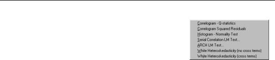
Residual Tests
EViews provides tests for serial correlation, normality, heteroskedasticity, and autoregressive conditional heteroskedasticity in the residuals from your estimated equation. Not all of these tests are available for every specification.
580—Chapter 19. Specification and Diagnostic Tests
Correlograms and Q-statistics
This view displays the autocorrelations and partial autocorrelations of the equation residuals up to the specified number of lags. Further details on these statistics and the Ljung-Box Q-statistics that are also computed are provided in Chapter 11, “Q-Statistics” on page 328.
This view is available for the residuals from least squares, two-stage least squares, nonlinear least squares and binary, ordered, censored, and count models. In calculating the probability values for the Q-statistics, the degrees of freedom are adjusted to account for estimated ARMA terms.
To display the correlograms and Q-statistics, push View/Residual Tests/Correlogram-Q- statistics on the equation toolbar. In the Lag Specification dialog box, specify the number of lags you wish to use in computing the correlogram.
Correlograms of Squared Residuals
This view displays the autocorrelations and partial autocorrelations of the squared residuals up to any specified number of lags and computes the Ljung-Box Q-statistics for the corresponding lags. The correlograms of the squared residuals can be used to check autoregressive conditional heteroskedasticity (ARCH) in the residuals; see also “ARCH LM Test” on page 582, below.
If there is no ARCH in the residuals, the autocorrelations and partial autocorrelations should be zero at all lags and the Q-statistics should not be significant; see Chapter 11, page 326, for a discussion of the correlograms and Q-statistics.
This view is available for equations estimated by least squares, two-stage least squares, and nonlinear least squares estimation. In calculating the probability for Q-statistics, the degrees of freedom are adjusted for the inclusion of ARMA terms.
To display the correlograms and Q-statistics of the squared residuals, push View/Residual Tests/Correlogram Squared Residuals on the equation toolbar. In the Lag Specification dialog box that opens, specify the number of lags over which to compute the correlograms.
Histogram and Normality Test
This view displays a histogram and descriptive statistics of the residuals, including the Jarque-Bera statistic for testing normality. If the residuals are normally distributed, the histogram should be bell-shaped and the Jarque-Bera statistic should not be significant; see Chapter 11, page 312, for a discussion of the Jarque-Bera test. This view is available for residuals from least squares, two-stage least squares, nonlinear least squares, and binary, ordered, censored, and count models.

Residual Tests—581
To display the histogram and Jarque-Bera statistic, select View/Residual Tests/HistogramNormality. The Jarque-Bera statistic has a χ2 distribution with two degrees of freedom under the null hypothesis of normally distributed errors.
Serial Correlation LM Test
This test is an alternative to the Q-statistics for testing serial correlation. The test belongs to the class of asymptotic (large sample) tests known as Lagrange multiplier (LM) tests.
Unlike the Durbin-Watson statistic for AR(1) errors, the LM test may be used to test for higher order ARMA errors and is applicable whether or not there are lagged dependent variables. Therefore, we recommend its use (in preference to the DW statistic) whenever you are concerned with the possibility that your errors exhibit autocorrelation.
The null hypothesis of the LM test is that there is no serial correlation up to lag order p , where p is a pre-specified integer. The local alternative is ARMA(r, q ) errors, where the number of lag terms p =max(r, q ). Note that this alternative includes both AR( p ) and MA(p ) error processes, so that the test may have power against a variety of alternative autocorrelation structures. See Godfrey (1988), for further discussion.
The test statistic is computed by an auxiliary regression as follows. First, suppose you have estimated the regression;
yt = Xtβ + t |
|
(19.13) |
||
where b are the estimated coefficients and |
are the errors. The test statistic for lag order |
|||
p is based on the auxiliary regression for the residuals e |
ˆ |
|
||
= y − Xβ : |
|
|||
|
p |
|
|
|
et = Xtγ + |
Σ αset − s + vt . |
(19.14) |
||
s = 1
Following the suggestion by Davidson and MacKinnon (1993), EViews sets any presample values of the residuals to 0. This approach does not affect the asymptotic distribution of the statistic, and Davidson and MacKinnon argue that doing so provides a test statistic which has better finite sample properties than an approach which drops the initial observations.
This is a regression of the residuals on the original regressors X and lagged residuals up to order p . EViews reports two test statistics from this test regression. The F-statistic is an omitted variable test for the joint significance of all lagged residuals. Because the omitted variables are residuals and not independent variables, the exact finite sample distribution of the F-statistic under H0 is still not known, but we present the F-statistic for comparison purposes.
The Obs*R-squared statistic is the Breusch-Godfrey LM test statistic. This LM statistic is computed as the number of observations, times the (uncentered) R2 from the test regres-

582—Chapter 19. Specification and Diagnostic Tests
sion. Under quite general conditions, the LM test statistic is asymptotically distributed as a
χ2(p) .
The serial correlation LM test is available for residuals from either least squares or twostage least squares estimation. The original regression may include AR and MA terms, in which case the test regression will be modified to take account of the ARMA terms. Testing in 2SLS settings involves additional complications, see Wooldridge (1990) for details.
To carry out the test, push View/Residual Tests/Serial Correlation LM Test… on the equation toolbar and specify the highest order of the AR or MA process that might describe the serial correlation. If the test indicates serial correlation in the residuals, LS standard errors are invalid and should not be used for inference.
ARCH LM Test
This is a Lagrange multiplier (LM) test for autoregressive conditional heteroskedasticity (ARCH) in the residuals (Engle 1982). This particular specification of heteroskedasticity was motivated by the observation that in many financial time series, the magnitude of residuals appeared to be related to the magnitude of recent residuals. ARCH in itself does not invalidate standard LS inference. However, ignoring ARCH effects may result in loss of efficiency; see Chapter 20 for a discussion of estimation of ARCH models in EViews.
The ARCH LM test statistic is computed from an auxiliary test regression. To test the null hypothesis that there is no ARCH up to order q in the residuals, we run the regression:
2 |
|
q |
2 |
+ vt , |
|
et |
= β0 + |
Σ βset − s |
(19.15) |
||
s = 1
where e is the residual. This is a regression of the squared residuals on a constant and lagged squared residuals up to order q . EViews reports two test statistics from this test regression. The F-statistic is an omitted variable test for the joint significance of all lagged squared residuals. The Obs*R-squared statistic is Engle’s LM test statistic, computed as the number of observations times the R2 from the test regression. The exact finite sample distribution of the F-statistic under H0 is not known but the LM test statistic is asymptotically distributed χ2(q) under quite general conditions. The ARCH LM test is available for equations estimated by least squares, two-stage least squares, and nonlinear least squares.
To carry out the test, push View/Residual Tests/ARCH LM Test… on the equation toolbar and specify the order of ARCH to be tested against.
White's Heteroskedasticity Test
This is a test for heteroskedasticity in the residuals from a least squares regression (White, 1980). Ordinary least squares estimates are consistent in the presence of heteroskedasticity, but the conventional computed standard errors are no longer valid. If you find evi-

Residual Tests—583
dence of heteroskedasticity, you should either choose the robust standard errors option to correct the standard errors (see “Heteroskedasticity Consistent Covariances (White)” on page 472) or you should model the heteroskedasticity to obtain more efficient estimates using weighted least squares.
White’s test is a test of the null hypothesis of no heteroskedasticity against heteroskedasticity of some unknown general form. The test statistic is computed by an auxiliary regression, where we regress the squared residuals on all possible (nonredundant) cross products of the regressors. For example, suppose we estimated the following regression:
yt = b1 + b2xt + b3zt + et |
(19.16) |
where the b are the estimated parameters and e the residual. The test statistic is then based on the auxiliary regression:
et2 = α0 + α1xt + α2zt + α3xt2 + α4zt2 + α5xtzt + vt . |
(19.17) |
EViews reports two test statistics from the test regression. The F-statistic is an omitted variable test for the joint significance of all cross products, excluding the constant. It is presented for comparison purposes.
The Obs*R-squared statistic is White’s test statistic, computed as the number of observations times the centered R2 from the test regression. The exact finite sample distribution of the F-statistic under H0 is not known, but White’s test statistic is asymptotically distributed as a χ2 with degrees of freedom equal to the number of slope coefficients (excluding the constant) in the test regression.
White also describes this approach as a general test for model misspecification, since the null hypothesis underlying the test assumes that the errors are both homoskedastic and independent of the regressors, and that the linear specification of the model is correct. Failure of any one of these conditions could lead to a significant test statistic. Conversely, a non-significant test statistic implies that none of the three conditions is violated.
When there are redundant cross-products, EViews automatically drops them from the test regression. For example, the square of a dummy variable is the dummy variable itself, so that EViews drops the squared term to avoid perfect collinearity.
To carry out White’s heteroskedasticity test, select View/Residual Tests/White Heteroskedasticity. EViews has two options for the test: cross terms and no cross terms. The cross terms version of the test is the original version of White’s test that includes all of the cross product terms (in the example above, xtzt ). However, with many right-hand side variables in the regression, the number of possible cross product terms becomes very large so that it may not be practical to include all of them. The no cross terms option runs the test regression using only squares of the regressors.