


322—Chapter 11. Series
F = sL2 ⁄ sS2 |
(11.14) |
where s2g is the variance in subgroup g . This F-statistic has an F-distribution with nL − 1 numerator degrees of freedom and nS − 1 denominator degrees of freedom under the null hypothesis of equal variance and independent normal samples.
•Siegel-Tukey test. This test statistic is reported only for tests with two subgroups ( G = 2) . The test assumes the two subgroups are independent and have equal
medians. The test statistic is computed using the same steps as the Kruskal-Wallis test described above for the median equality tests (“Median (Distribution) Equality Tests” on page 320), with a different assignment of ranks. The ranking for the SiegelTukey test alternates from the lowest to the highest value for every other rank. The Siegel-Tukey test first orders all observations from lowest to highest. Next, assign rank 1 to the lowest value, rank 2 to the highest value, rank 3 to the second highest value, rank 4 to the second lowest value, rank 5 to the third lowest value, and so on. EViews reports the normal approximation to the Siegel-Tukey statistic with a continuity correction (Sheskin, 1997, pp. 196–207).
•Bartlett test. This test compares the logarithm of the weighted average variance with the weighted sum of the logarithms of the variances. Under the joint null hypothesis
that the subgroup variances are equal and that the sample is normally distributed, the test statistic is approximately distributed as a χ2 with G = 1 degrees of free-
dom. Note, however, that the joint hypothesis implies that this test is sensitive to departures from normality. EViews reports the adjusted Bartlett statistic. For details, see Sokal and Rohlf (1995) and Judge, et al. (1985).
•Levene test. This test is based on an analysis of variance (ANOVA) of the absolute
difference from the mean. The F-statistic for the Levene test has an approximate F- distribution with G = 1 numerator degrees of freedom and N − G denominator
degrees of freedom under the null hypothesis of equal variances in each subgroup (Levene, 1960).
•Brown-Forsythe (modified Levene) test. This is a modification of the Levene test in which we replace the absolute mean difference with the absolute median difference. The Brown-Forsythe test appears to be a superior in terms of robustness and power (Conover, et al. (1981), Brown and Forsythe (1974a, 1974b), Neter, et al. (1996)).
Distribution Graphs
These views display various graphs that characterize the empirical distribution of the series. A detailed description of these views may also be found in Chapter 13, “Statistical Graphs from Series and Groups”, beginning on page 391.

Distribution Graphs—323
CDF-Survivor-Quantile
This view plots the empirical cumulative distribution, survivor, and quantile functions of the series together with plus/minus two standard error bands. EViews provides a number of alternative methods for performing these computations.
Quantile-Quantile
The quantile-quantile (QQ)-plot is a simple yet powerful tool for comparing two distributions. This view plots the quantiles of the chosen series against the quantiles of another series or a theoretical distribution.
Kernel Density
This view plots the kernel density estimate of the distribution of the series. The simplest nonparametric density estimate of a distribution of a series is the histogram. The histogram, however, is sensitive to the choice of origin and is not continuous. The kernel density estimator replaces the “boxes” in a histogram by “bumps” that are smooth (Silverman 1986). Smoothing is done by putting less weight on observations that are further from the point being evaluated.
EViews provides a number of kernel choices as well as control over bandwidth selection and computational method.
Empirical Distribution Tests
EViews provides built-in Kolmogorov-Smirnov, Lilliefors, Cramer-von Mises, AndersonDarling, and Watson empirical distribution tests. These tests are based on the comparison between the empirical distribution and the specified theoretical distribution function. For a general description of empirical distribution function testing, see D’Agostino and Stephens (1986).
You can test whether your series is normally distributed, or whether it comes from, among others, an exponential, extreme value, logistic, chi-square, Weibull, or gamma distribution. You may provide parameters for the distribution, or EViews will estimate the parameters for you.
To carry out the test, simply double click on the series and select View/Distribution/ Empirical Distribution Tests... from the series window.
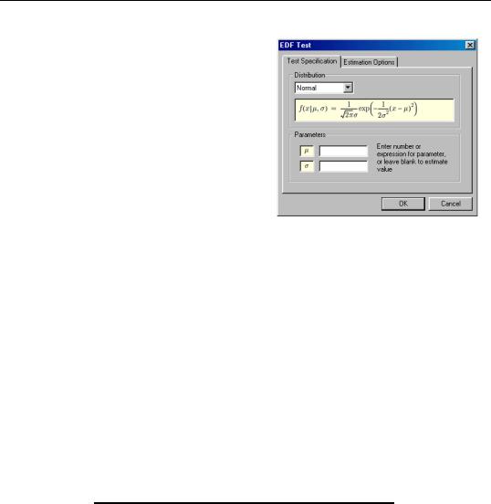
324—Chapter 11. Series
There are two tabs in the dialog. The Test Specification tab allows you to specify the parametric distribution against which you want to test the empirical distribution of the series. Simply select the distribution of interest from the drop-down menu. The small display window will change to show you the parameterization of the specified distribution.
You can specify the values of any known parameters in the edit field or fields. If you leave any field blank, EViews will estimate the corresponding parameter using the data contained in the series.
The Estimation Options tab provides control over any iterative estimation that is required. You should not need to use this tab unless the output indicates failure in the estimation process. Most of the options in this tab should be self-explanatory. If you select User-spec- ified starting values, EViews will take the starting values from the C coefficient vector.
It is worth noting that some distributions have positive probability on a restricted domain. If the series data take values outside this domain, EViews will report an out-of-range error. Similarly, some of the distributions have restrictions on domain of the parameter values. If you specify a parameter value that does not satisfy this restriction, EViews will report an error message.
The output from this view consists of two parts. The first part displays the test statistics and associated probability values.
Empirical Distribution Test for DPOW2
Hypothesis: Normal
Date: 01/09/01 Time: 09:11
Sample: 1 1000
Included observations: 1000
Method |
Value |
Adj. Value |
Probability |
|
|
|
|
Lilliefors (D) |
0.294098 |
NA |
0.0000 |
Cramer-von Mises (W2) |
27.89617 |
27.91012 |
0.0000 |
Watson (U2) |
25.31586 |
25.32852 |
0.0000 |
Anderson-Darling (A2) |
143.6455 |
143.7536 |
0.0000 |
|
|
|
|
Here, we show the output from a test for normality where both the mean and the variance are estimated from the series data. The first column, “Value”, reports the asymptotic test statistics while the second column, “Adj. Value”, reports test statistics that have a finite

One-Way Tabulation—325
sample correction or adjusted for parameter uncertainty (in case the parameters are estimated). The third column reports p-value for the adjusted statistics.
All of the reported EViews p-values will account for the fact that parameters in the distribution have been estimated. In cases where estimation of parameters is involved, the distributions of the goodness-of-fit statistics are non-standard and distribution dependent, so that EViews may report a subset of tests and/or only a range of p-value. In this case, for example, EViews reports the Lilliefors test statistic instead of the Kolmogorov statistic since the parameters of the normal have been estimated. Details on the computation of the test statistics and the associated p-values may be found in Anderson and Darling (1952, 1954), Lewis (1961), Durbin (1970), Dallal and Wilkinson (1986), Davis and Stephens (1989), Csörgö and Faraway (1996) and Stephens (1986).
Method: Maximum Likelihood - d.f. corrected (Exact Solution)
Parameter |
Value |
Std. Error |
z-Statistic |
Prob. |
|
|
|
|
|
MU |
0.142836 |
0.015703 |
9.096128 |
0.0000 |
SIGMA |
0.496570 |
0.011109 |
44.69899 |
0.0000 |
|
|
|
|
|
Log likelihood |
-718.4084 |
Mean dependent var. |
0.142836 |
|
No. of Coefficients |
2 |
S.D. dependent var. |
0.496570 |
|
|
|
|
|
|
The second part of the output table displays the parameter values used to compute the theoretical distribution function. Any parameters that are specified to estimate are estimated by maximum likelihood (for the normal distribution, the estimate of the standard deviation is degree of freedom corrected if the mean is not specified a priori). For parameters that do not have a closed form analytic solution, the likelihood function is maximized using analytic first and second derivatives. These estimated parameters are reported with a standard error and p-value based on the asymptotic normal distribution.
One-Way Tabulation
This view tabulates the series in ascending order, optionally displaying the counts, percentage counts, and cumulative counts. When you select View/One-Way Tabulation… the Tabulate Series dialog box will be displayed.
The Output options control which statistics to display in the table. You should specify the NA handling and the grouping options as described above in the discussion of “Stats by Classification” on page 312.
Cross-tabulation ( n -way tabulation) is also available as a group view. See “N-Way Tabulation” on page 381 for details.