658—Chapter 21. Discrete and Limited Dependent Variable Models

Note that the header information indicates that the model is a truncated specification, and that the sample information at the bottom of the screen shows that there are no left and right censored observations.

Count Models

Count models are employed when y takes integer values that represent the number of events that occur—examples of count data include the number of patents filed by a company, and the number of spells of unemployment experienced over a fixed time interval.

EViews provides support for the estimation of several models of count data. In addition to the standard poisson and negative binomial maximum likelihood (ML) specifications, EViews provides a number of quasi-maximum likelihood (QML) estimators for count data.

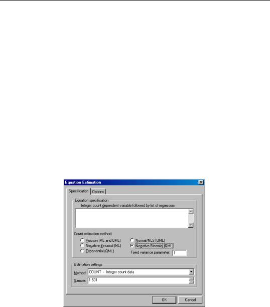
Estimating Count Models in EViews

To estimate a count data model, select Quick/Estimate Equation… from the main menu, and select COUNT as the estimation method. EViews displays the count estimation dialog into which you will enter the dependent and explanatory variable regressors, select a type of count model, and if desired, set estimation options.

There are three parts to the specification of the count model:

•In the upper edit field, you should list the dependent variable and the independent variables. You must specify your model by list. The list of explanatory variables specifies a model for the conditional mean of the dependent variable:

Count Models—659

•Next, click on Options and, if desired, change the default estimation algorithm, convergence criterion, starting values, and method of computing the coefficient covariance.

•Lastly, select one of the entries listed under count estimation method, and if appropriate, specify a value for the variance parameter. Details for each method are provided in the following discussion.

Poisson Model

where yi is a non-negative integer valued random variable. The maximum likelihood estimator (MLE) of the parameter β is obtained by maximizing the log likelihood function:

i = 1

Provided the conditional mean function is correctly specified and the conditional distribu-

The Poisson assumption imposes restrictions that are often violated in empirical applications. The most important restriction is the equality of the (conditional) mean and variance:

If the mean-variance equality does not hold, the model is misspecified. EViews provides a number of other estimators for count data which relax this restriction.

We note here that the Poisson estimator may also be interpreted as a quasi-maximum likelihood estimator. The implications of this result are discussed below.

Negative Binomial (ML)

One common alternative to the Poisson model is to estimate the parameters of the model using maximum likelihood of a negative binomial specification. The log likelihood for the negative binomial distribution is given by:

660—Chapter 21. Discrete and Limited Dependent Variable Models

i= 1

−( yi + 1 ⁄ η2) log ( 1 + η2m( xi, β) )

+ log Γ( yi + 1 ⁄ η2) −log ( yi!) − log Γ( 1 ⁄ η2)

where η2 is a variance parameter to be jointly estimated with the conditional mean parameters β . EViews estimates the log of η2 , and labels this parameter as the “SHAPE” parameter in the output. Standard errors are computed using the inverse of the information matrix.

The negative binomial distribution is often used when there is overdispersion in the data, so that v( xi, β) > m( xi, β) , since the following moment conditions hold:

E( yi xi, β) = m( xi, β)

(21.44)

var( yi xi, β) = m( xi, β) ( 1 + η2m( xi, β) )

η2 is therefore a measure of the extent to which the conditional variance exceeds the conditional mean.

Consistency and efficiency of the negative binomial ML requires that the conditional distribution of y be negative binomial.

Quasi-maximum Likelihood (QML)

We can perform maximum likelihood estimation under a number of alternative distributional assumptions. These quasi-maximum likelihood (QML) estimators are robust in the sense that they produce consistent estimates of the parameters of a correctly specified conditional mean, even if the distribution is incorrectly specified.

This robustness result is exactly analogous to the situation in ordinary regression, where the normal ML estimator (least squares) is consistent, even if the underlying error distribution is not normally distributed. In ordinary least squares, all that is required for consistency is a correct specification of the conditional mean m( xi, β) = xi′β . For QML count models, all that is required for consistency is a correct specification of the conditional mean m( xi, β) .

The estimated standard errors computed using the inverse of the information matrix will not be consistent unless the conditional distribution of y is correctly specified. However, it is possible to estimate the standard errors in a robust fashion so that we can conduct valid inference, even if the distribution is incorrectly specified.