

- •Analysis and Application of Analog Electronic Circuits to Biomedical Instrumentation
- •Dedication
- •Preface
- •Reader Background
- •Rationale
- •Description of the Chapters
- •Features
- •The Author
- •Table of Contents
- •1.1 Introduction
- •1.2 Sources of Endogenous Bioelectric Signals
- •1.3 Nerve Action Potentials
- •1.4 Muscle Action Potentials
- •1.4.1 Introduction
- •1.4.2 The Origin of EMGs
- •1.5 The Electrocardiogram
- •1.5.1 Introduction
- •1.6 Other Biopotentials
- •1.6.1 Introduction
- •1.6.2 EEGs
- •1.6.3 Other Body Surface Potentials
- •1.7 Discussion
- •1.8 Electrical Properties of Bioelectrodes
- •1.9 Exogenous Bioelectric Signals
- •1.10 Chapter Summary
- •2.1 Introduction
- •2.2.1 Introduction
- •2.2.4 Schottky Diodes
- •2.3.1 Introduction
- •2.4.1 Introduction
- •2.5.1 Introduction
- •2.5.5 Broadbanding Strategies
- •2.6 Photons, Photodiodes, Photoconductors, LEDs, and Laser Diodes
- •2.6.1 Introduction
- •2.6.2 PIN Photodiodes
- •2.6.3 Avalanche Photodiodes
- •2.6.4 Signal Conditioning Circuits for Photodiodes
- •2.6.5 Photoconductors
- •2.6.6 LEDs
- •2.6.7 Laser Diodes
- •2.7 Chapter Summary
- •Home Problems
- •3.1 Introduction
- •3.2 DA Circuit Architecture
- •3.4 CM and DM Gain of Simple DA Stages at High Frequencies
- •3.4.1 Introduction
- •3.5 Input Resistance of Simple Transistor DAs
- •3.7 How Op Amps Can Be Used To Make DAs for Medical Applications
- •3.7.1 Introduction
- •3.8 Chapter Summary
- •Home Problems
- •4.1 Introduction
- •4.3 Some Effects of Negative Voltage Feedback
- •4.3.1 Reduction of Output Resistance
- •4.3.2 Reduction of Total Harmonic Distortion
- •4.3.4 Decrease in Gain Sensitivity
- •4.4 Effects of Negative Current Feedback
- •4.5 Positive Voltage Feedback
- •4.5.1 Introduction
- •4.6 Chapter Summary
- •Home Problems
- •5.1 Introduction
- •5.2.1 Introduction
- •5.2.2 Bode Plots
- •5.5.1 Introduction
- •5.5.3 The Wien Bridge Oscillator
- •5.6 Chapter Summary
- •Home Problems
- •6.1 Ideal Op Amps
- •6.1.1 Introduction
- •6.1.2 Properties of Ideal OP Amps
- •6.1.3 Some Examples of OP Amp Circuits Analyzed Using IOAs
- •6.2 Practical Op Amps
- •6.2.1 Introduction
- •6.2.2 Functional Categories of Real Op Amps
- •6.3.1 The GBWP of an Inverting Summer
- •6.4.3 Limitations of CFOAs
- •6.5 Voltage Comparators
- •6.5.1 Introduction
- •6.5.2. Applications of Voltage Comparators
- •6.5.3 Discussion
- •6.6 Some Applications of Op Amps in Biomedicine
- •6.6.1 Introduction
- •6.6.2 Analog Integrators and Differentiators
- •6.7 Chapter Summary
- •Home Problems
- •7.1 Introduction
- •7.2 Types of Analog Active Filters
- •7.2.1 Introduction
- •7.2.3 Biquad Active Filters
- •7.2.4 Generalized Impedance Converter AFs
- •7.3 Electronically Tunable AFs
- •7.3.1 Introduction
- •7.3.3 Use of Digitally Controlled Potentiometers To Tune a Sallen and Key LPF
- •7.5 Chapter Summary
- •7.5.1 Active Filters
- •7.5.2 Choice of AF Components
- •Home Problems
- •8.1 Introduction
- •8.2 Instrumentation Amps
- •8.3 Medical Isolation Amps
- •8.3.1 Introduction
- •8.3.3 A Prototype Magnetic IsoA
- •8.4.1 Introduction
- •8.6 Chapter Summary
- •9.1 Introduction
- •9.2 Descriptors of Random Noise in Biomedical Measurement Systems
- •9.2.1 Introduction
- •9.2.2 The Probability Density Function
- •9.2.3 The Power Density Spectrum
- •9.2.4 Sources of Random Noise in Signal Conditioning Systems
- •9.2.4.1 Noise from Resistors
- •9.2.4.3 Noise in JFETs
- •9.2.4.4 Noise in BJTs
- •9.3 Propagation of Noise through LTI Filters
- •9.4.2 Spot Noise Factor and Figure
- •9.5.1 Introduction
- •9.6.1 Introduction
- •9.7 Effect of Feedback on Noise
- •9.7.1 Introduction
- •9.8.1 Introduction
- •9.8.2 Calculation of the Minimum Resolvable AC Input Voltage to a Noisy Op Amp
- •9.8.5.1 Introduction
- •9.8.5.2 Bridge Sensitivity Calculations
- •9.8.7.1 Introduction
- •9.8.7.2 Analysis of SNR Improvement by Averaging
- •9.8.7.3 Discussion
- •9.10.1 Introduction
- •9.11 Chapter Summary
- •Home Problems
- •10.1 Introduction
- •10.2 Aliasing and the Sampling Theorem
- •10.2.1 Introduction
- •10.2.2 The Sampling Theorem
- •10.3 Digital-to-Analog Converters (DACs)
- •10.3.1 Introduction
- •10.3.2 DAC Designs
- •10.3.3 Static and Dynamic Characteristics of DACs
- •10.4 Hold Circuits
- •10.5 Analog-to-Digital Converters (ADCs)
- •10.5.1 Introduction
- •10.5.2 The Tracking (Servo) ADC
- •10.5.3 The Successive Approximation ADC
- •10.5.4 Integrating Converters
- •10.5.5 Flash Converters
- •10.6 Quantization Noise
- •10.7 Chapter Summary
- •Home Problems
- •11.1 Introduction
- •11.2 Modulation of a Sinusoidal Carrier Viewed in the Frequency Domain
- •11.3 Implementation of AM
- •11.3.1 Introduction
- •11.3.2 Some Amplitude Modulation Circuits
- •11.4 Generation of Phase and Frequency Modulation
- •11.4.1 Introduction
- •11.4.3 Integral Pulse Frequency Modulation as a Means of Frequency Modulation
- •11.5 Demodulation of Modulated Sinusoidal Carriers
- •11.5.1 Introduction
- •11.5.2 Detection of AM
- •11.5.3 Detection of FM Signals
- •11.5.4 Demodulation of DSBSCM Signals
- •11.6 Modulation and Demodulation of Digital Carriers
- •11.6.1 Introduction
- •11.6.2 Delta Modulation
- •11.7 Chapter Summary
- •Home Problems
- •12.1 Introduction
- •12.2.1 Introduction
- •12.2.2 The Analog Multiplier/LPF PSR
- •12.2.3 The Switched Op Amp PSR
- •12.2.4 The Chopper PSR
- •12.2.5 The Balanced Diode Bridge PSR
- •12.3 Phase Detectors
- •12.3.1 Introduction
- •12.3.2 The Analog Multiplier Phase Detector
- •12.3.3 Digital Phase Detectors
- •12.4 Voltage and Current-Controlled Oscillators
- •12.4.1 Introduction
- •12.4.2 An Analog VCO
- •12.4.3 Switched Integrating Capacitor VCOs
- •12.4.6 Summary
- •12.5 Phase-Locked Loops
- •12.5.1 Introduction
- •12.5.2 PLL Components
- •12.5.3 PLL Applications in Biomedicine
- •12.5.4 Discussion
- •12.6 True RMS Converters
- •12.6.1 Introduction
- •12.6.2 True RMS Circuits
- •12.7 IC Thermometers
- •12.7.1 Introduction
- •12.7.2 IC Temperature Transducers
- •12.8 Instrumentation Systems
- •12.8.1 Introduction
- •12.8.5 Respiratory Acoustic Impedance Measurement System
- •12.9 Chapter Summary
- •References

Examples of Special Analog Circuits and Systems |
511 |
1 kΩ |
CHSOA |
+ |
8.66 kΩ |
(0) |
Vo = 100 mV/oC |
+ 2.5 V |
||
|
|
− |
1 µA/oK |
97.6 kΩ 5 kΩ |
|
T AD592
−15 V
FIGURE 12.36
A simple op amp current-to-voltage converter that converts the current output of an AD592 temperature sensor to 100 mV/∞C.
calibrate the amplifier exactly so that it has zero gain and offset error at the design temperature, e.g., 37∞C.
Note that National Semiconductor also makes IC temperature sensors. The National LM135 series of sensors behave as temperature-controlled voltage drops (much like a zener diode). They give 10 mV/K drop with approximately 1-Ω dynamic resistance for DC currents ranging from 400 μA to 5 mA. They cover a wide, −55 to +150∞C range. The National LM35 precision Celsius temperature sensor is a three-terminal device that outputs an EMF of 10 mV/∞C over a −55 to +150∞C range, given a supply voltage from 4 to
30VDC.
12.8Instrumentation Systems
12.8.1Introduction
The previous sections of this chapter have described and analyzed the characteristics of selected ICs useful in designing biomedical instrumentation systems. This section focuses on examples of biomedical instrumentation systems taken from the research of the author and some of his graduate students. In each system, op amps are used extensively for various linear and nonlinear subsystems.
12.8.2A Self-Nulling Microdegree Polarimeter
A polarimeter is an instrument used to measure the angle of rotation of linearly polarized light when it is passed through an optically active material. There are many types of polarimeters as well as a number of optically active
© 2004 by CRC Press LLC
512 |
Analysis and Application of Analog Electronic Circuits |
substances found in living systems; probably the most important is dissolved D-glucose. Clear biological liquids such as urine, blood plasma, and the aqueous humor of the eyes contain dissolved D-glucose with a molar concentration in proportion to the blood glucose concentration (Northrop, 2002). Using polarimetry, D-glucose concentration can be measured by the simple relation:
φ = [α]T |
C L degrees |
(12.80) |
λ |
|
|
where φ is the measured optical rotation of linearly polarized light (LPL) of wavelength λ passed through a sample chamber of length L containing the optically active analyte at concentration C and temperature T.
The constant [α]λT is called the specific optical rotation of the analyte; its units are generally in degrees per (optical path length unit ∞ concentration unit). [α]λT for D-glucose in 25∞C water and at 512 nm is 0.0695 millidegrees/(cm ∞ g/dl). Thus, the optical rotation of a 1-g/l solution of D-glucose in a 10-cm cell is 69.5 millidegrees. Note that [α]λT can have either sign, depending on the analyte; if N optically active substances are present in the sample chamber, the net optical rotation is given by superposition:
N |
|
|
φ = L [α]λTk Ck |
(12.81) |
|
k = |
1 |
|
To describe how a polarimeter works, one must first describe what is meant by linearly polarized light. When light from an incoherent source such as a tungsten lamp is treated as an electromagnetic wave phenomenon (rather than photons), the propagating radiation is composed of a broad spectrum of wavelengths and polarization states. To facilitate the description of LPL, examine a monochromatic ray propagating in the z-direction at the speed of light in the medium in which it is traveling. This velocity in the z-direction is v = c/n m/s; c is the velocity of light in vacuo and n is the refractive index of the propagation medium (generally >1.0). A beam of monochromatic light can have a variety of polarization states, including random (unpolarized), circular (CW or CCW), elliptical, and linear (Balanis, 1989). Figure 12.37 illustrates an LPL ray in which the E-vector propagates entirely in the x–z plane, and its orthogonal By–vector lies in the y–z plane; E and B are inphase and both vectors are functions of time and distance.
For the Ex(t, z) vector:
2 πc |
|
2 π |
˘ |
|
||
Ex (t, z) = Eox cos |
|
t − |
|
z˙ |
(12.82) |
|
λ |
λ |
|||||
|
|
˚ |
|
|||
Note that the E-vector need not lie in the x–z plane; its plane of propagation can be tilted some angle θ with respect to the x-axis and still propagate in
© 2004 by CRC Press LLC

Examples of Special Analog Circuits and Systems |
513 |
||
|
x |
|
|
|
Eox |
λ |
|
|
Ex |
|
|
|
|
z |
|
|
P |
|
|
y |
By |
v = c/n |
|
Boy |
|||
|
|
||
FIGURE 12.37
Diagram of a linearly polarized electromagnetic wave (e.g., light) propagating in the z direction. By(t) is orthogonal in space to Ex(t).
the z-direction (the orthogonal B-vector is rotated θ with respect to the y-axis). When describing LPL, examine the positive maximums of the E-vector and make a vector with this maximum and at an angle θ with the x-axis in the x–y plane.
Figure 12.38 illustrates what happens to LPL of wavelength λ passing though a sample chamber containing an optically active analyte. Polarizer P1 converts the input light to a linearly polarized beam that is passed through the sample chamber. As the result of the interaction of the light with the optically active solute, the emergent LPL ray is rotated by an angle, θ. In this figure, the analyte is dextrorotary, that is, the emergent E-vector, E2, is rotated clockwise when viewed in the direction of propagation (along the +z-axis). (D-glucose is dextrorotary.)
To measure the optical rotation of the sample, a second polarizer, P2, is rotated until a null in the light intensity striking the photosensor is noted (in its simplest form, the photosensor can be a human’s eye). This null is when P2’s pass axis is orthogonal to E2 – θ . Because polarizer P1 is set with its pass axis aligned with the x-axis (i.e., at 0∞) it is easy to find θ, and then the concentration of the optically active analyte, [G]. In the simple polarimeter of Figure 12.38, and other polarimeters, the polarizers are generally made from calcite crystals (Glan calcite) and have extinction ratios of approximately 104. (Extinction ratio is the ratio of LPL intensity passing through the polarizer, when the LPL’s polarization axis is aligned with the polarizer’s pass axis, to the intensity of the emergent beam when the polarization axis is made 90∞ (is orthogonal) to the polarizer’s axis.)
To make an electronic polarimeter, an electrical means of nulling the polarimeter output is needed, as opposed to rotating P2 around the z-axis physically. One means of generating an electrically controlled optical rotation is to use the Faraday magneto-optical effect. Figure 12.39 illustrates a Faraday rotator (FR). An FR has two major components: (1) a magneto optically active medium. Many transparent gasses, liquids and solids exhibit magneto-opti- cal activity, e.g., a lead glass rod with optically flat ends or a glass test
© 2004 by CRC Press LLC

514 |
Analysis and Application of Analog Electronic Circuits |
x
E1 Sample cuvette
PAx 
P1
Laser
z
y
Optically-active medium
L
 x
x
θ = [α]Tλ L [G]  x
x
 E2
E2
θ
P2
Photosensor
z |
|
z |
E3 |
y |
E3 y |
|
|
|
|
|
PAy |
E3 = E2 sin(θ) |
Null at (θ + 90o) |
|
I3 E22 sin2(θ)
FIGURE 12.38
Diagram showing the rotation of the polarization axis of the incident E1 vector by passing the LPL through an optically active medium of length L. The system is a polarimeter: When the pass axis of linear polarizer P2 is rotated by angle θ + 90∞, a null is observed in the output intensity, I3. Thus, θ can be measured.
x |
Ic |
x |
|
|
(Optical |
||
|
|
||
Ein |
|
rotation) |
|
Faraday medium |
θ |
|
|
|
Eout |
||
|
|
|
|
|
z |
|
z |
LPL |
|
|
|
|
|
|
|
(λ) |
|
D |
|
y |
y |
|
|
N-turn solenoid |
Ic |
|
l |
|
_
θ = V(λ, T) B l
FIGURE 12.39
Diagram of a Faraday rotator (FR). The z-axis magnetic field component from the currentcarrying solenoid interacts with the Faraday medium to cause optical rotation of LPL passing through the medium in the z-direction.
chamber with optically flat ends containing a gas or liquid can be used. (2) A solenoidal coil wound around the rod or test chamber that generates an axial magnetic field, B, inside the rod or chamber collinear with the entering LPL beam. The exiting LPL beam undergoes optical rotation according to the simple Faraday relation (Hecht, 1987):
θm = V(λ, T) |
|
z l |
(12.83) |
B |
© 2004 by CRC Press LLC

Examples of Special Analog Circuits and Systems |
515 |
where θm is the Faraday optical rotation in degrees, V(λ, T) is the magneto optically active material’s Verdet constant, having units of degrees/(Tesla meter).
Verdet constants are given in a variety of challenging units, such as 10−3 min of arc/(gauss.cm). `Bz is the average axial flux density collinear with the optical path and l is the length of the path in which the LPL is exposed to the axial B field. A material’s Verdet constant increases with decreasing wavelength, and with increasing temperature. When a Verdet constant is specified, the wavelength and temperature at which it was measured must be given. For example, the Verdet constant of distilled water at 20∞C and 578 nm is 218.3∞/(Tm) (Hecht, 1987, Chapter 8). This value may appear large, but the length of the test chamber on which the solenoid is wound is 10 cm = 10−1 m and 1 T = 104 G, so actual rotations tend to be < ±5∞. The Verdet constant for lead glass under the same conditions is about six times larger. Not all Verdet constants are positive; for example, an aqueous solution of ferric chloride and solid amber have negative Verdet constants.
Two well-known formulas for axial B inside a solenoid follow (Krauss, 1953). At the center of the solenoid, on its axis:
Bz = |
μNI |
tesla |
(12.84) |
|
4R2 + l2 |
||||
|
|
|
At either end of the solenoid, on its axis:
Bz |
= |
|
μNI |
tesla |
(12.85) |
|
R2 + l2 |
||||
|
2 |
|
|
||
It can be shown, by averaging over l, that Bz over the length l of the solenoid is approximately:
|
|
|
3μNI |
|
3μNI |
tesla, when I 2R |
(12.86) |
B |
|
||||||
|
|
|
|||||
z |
4 |
4R2 + I2 |
|
4l |
|
||
|
|
|
|
||||
It should be clear that a Faraday rotator can be used to null a simple polarimeter electrically. See Figure 12.40 for an illustration of a simple dc electrically nulled polarimeter. The dc FR current is varied until the output photosensor registers a null (E4 = 0). At null, the optical rotation from the FR is equal and opposite to the optical rotation from the optically active analyte. Thus:
V(λ, T) |
3μNI |
l = [α]T CL |
(12.87) |
4l |
λ |
|
|
and the concentration of OA analyte is: |
|
© 2004 by CRC Press LLC

516 |
|
|
Analysis and Application of Analog Electronic Circuits |
|||||
Extrema of E-vectors |
x |
|
|
x |
|
|
|
|
in x-y plane |
|
|
x |
|
|
|||
|
|
|
|
|
|
|||
x |
|
|
|
− φs |
θmo + φs = 0 |
|
|
|
|
|
|
θmo |
|
|
|
||
|
E1 |
|
|
E3 |
|
|
|
|
|
|
|
|
|
|
|
||
|
|
|
E2 |
|
|
|
|
|
|
z |
|
z z |
|
|
E4 |
= 0 |
z |
|
|
|
|
|
|
|||
A |
|
B |
|
|
C |
D |
|
|
y |
|
|
|
|
|
|||
|
|
y |
|
y |
|
y |
|
|
|
|
|
|
|
|
|||
|
P1 |
|
|
|
|
|
|
|
|
|
|
|
|
|
|
|
Ip |
|
|
A |
|
B |
C |
|
D |
|
Source |
|
|
|
|
L |
|
|
Sensor |
|
|
|
|
|
P2 |
|
|
|
|
|
|
|
|
|
|
|
|
|
|
|
FR |
|
Sample cuvette |
|
|
|
|
|
|
i |
Rotation φs = [α]λTLC |
|
|
|
|
|
|
|
|
|
|
|
|
|
FIGURE 12.40
A simple electrically nulled polarimeter. The optical rotation from the FR is made equal and opposite to the optical rotation of the sample to get a null.
= 3VμNI
C [ ] (12.88) 4 α L
Note that C is dependent on three well-known parameters (N, I, and L) and two that are less well known and temperature dependent (V and [α]). This type of operation yields accuracy in the tenths of a degree.
Figure 12.41 illustrates an improvement on the static polarimeter shown in Figure 12.40. Now an ac current is passed through the FR, causing the emergent polarization vector at point B to rock back and forth sinusoidally in the x–y plane at audio frequency fm = ωm 2π Hz. The maximum rocking angle is θmo. This rocking E2 vector is next passed through the optically active sample where, at any instant, the angle of E2 has the rotation φs added to it, as shown at point C. Next, the asymmetrically rocking E3 vector is passed through polarizer P2, which only passes the y-components of E3 as E4y at point D. Thus E4y(t) can be written:
E4y (t) = E4yo sin[φs + θmo sin(ωmt)] |
(12.89) |
The sinusoidal component in the sin[*] argument is from the audiofrequency polarization angle modulation. The instantaneous intensity of the light at D, i4(t), is proportional to E4y2 (t):
i4 (t) = E4yo2 [c εo 2]sin2 [φs + θmo sin(ωmt)] Watts m2 |
(12.90) |
© 2004 by CRC Press LLC
Examples of Special Analog Circuits and Systems |
|
517 |
|||
|
|
x |
x |
|
x |
|
|
|
|
|
|
|
|
|
φs |
|
|
x |
|
−θmo |
φs − θmo |
|
|
|
E1 |
θmo |
|
θmo + φs |
|
|
|
|
|
|
|
|
|
E2 |
E3 |
|
|
|
|
E2 |
E3 |
|
|
|
z |
z |
|
z |
z |
A |
|
B |
C |
|
D |
y |
|
|
|||
|
y |
|
|
|
|
|
|
|
|
E4 |
|
|
|
|
|
y |
|
|
|
P1 |
|
|
|
|
|
|
|
|
|
|
|
|
|
|
Ip |
|
|
A |
B |
C |
D |
Source |
|
|
L |
|
Sensor |
|
|
|
|
P2 |
|
|
|
|
|
|
|
|
|
FR |
Sample cuvette |
|
|
|
|
i |
Rotation φs = [α]λTLC |
|
|
FIGURE 12.41
An open-loop Gilham polarimeter. The input polarization angle is rocked back and forth by ±θmo degrees by passing ac current through the FR. See text for analysis.
Now, by trigonometric identity, sin2 (x) = ½ [1 − cos(2x)], yielding:
i4 (t) = E4yo2 [c εo 2]12 {1− cos[2φs + 2θmo sin(ωmt)]} |
(12.91) |
Because the angle argument of the cosine is small, i.e., 2(φs + θmo) <3∞, the approximation cos(x) (1 − x2/2) may be used. Assume the instantaneous
photosensor output voltage, vp(t), is proportional to i4(t), so: |
|
|
||||||||||||
vp (t) = KP i4 (t) |
|
|
|
|
|
|
|
|
|
|
(12.92) |
|||
|
|
2 |
|
|
|
|
|
|
2 |
2 |
2 |
|
÷ |
|
KP |
™ |
(c εo |
2)12 |
™ |
− |
− |
4φs |
+ 4θmo sin |
|
(ωmt)+ 8φsθmo sin(ωmt)˘™ |
||||
E4yo |
1 |
1 |
|
|
|
|
|
˙˝ |
||||||
|
|
|
2 |
|
||||||||||
|
™ |
|
|
|
™ |
|
|
|
|
|
|
|
˙™ |
|
|
© |
|
|
|
© |
|
|
|
|
|
|
|
|
˚˛ |
|
|
|
|
|
|
|
|
|
¬ |
|
|
|
|
|
|
vp (t) = KV [φs2 + θmo2 12 (1− cos(2ωmt))+ 2φsθmo sin(ωmt)] |
(12.93) |
||||||||||||
where KV = KP E4yo2 (c εo 2).
Thus the photosensor output voltage contains three components: (1) a dc component of no interest; (2) a double-frequency component with no information on φs; and (3) a fundamental frequency sinusoidal term whose peak
© 2004 by CRC Press LLC
518 |
Analysis and Application of Analog Electronic Circuits |
amplitude is proportional to φs. By using a high-pass filter, the dc components can be blocked; by using a phase-sensitive rectifier synchronized to the FR modulating current sinusoid at ωm, a dc signal proportional to φs can be recovered while rejecting the 2ωm sinusoidal term.
By feeding a dc current proportional to φs back into the FR, the system can be made closed loop and self-nulling. The first such feedback polarimeter was invented by Gilham in 1957; it has been improved and modified by various workers since then (Northrop, 2002; Cameron and Coté; 1997, Coté, Fox, and Northrop, 1992; Rabinovitch, March, and Adams, 1982). Instruments of this sort can resolve φs to better than ±20 microdegrees.
Browne, Nelson, and Northrop (1997) devised a feedback polarimetry system that has microdegree resolution and is designed to measure glucose in bioreactors. The system is illustrated in Figure 12.42. Before its design and operation are described, it is necessary to understand how a conventional Gilham-type closed-loop polarimeter works.
A conventional closed-loop polarization angle-modulated Gilham polarimeter is shown in Figure 12.43. The dc light source can be a laser or laser diode. (A 512-nm (green) diode laser was used.) The light from the laser is passed through a calcite Glan-laser polarizer, P1, to improve its degree of polarization, and then through the Faraday rotator. Two things happen in the FR: (1) the input LPL is polarization angle-modulated at frequency fm. θmo is made about 2∞. After passing through the sample, the angle modulation is no longer symmetrical around the y-axis because the optically active analyte’s rotation has been added to the modulation angle. As shown previously, this causes a fundamental frequency sinusoidal voltage to appear at the output of the high-pass filter (HPF) whose peak amplitude is proportional to the desired φs. The phase-sensitive rectifier and LPF output a dc voltage, VL, proportional to φs.
(2) VL is integrated and the dc integrator output, Vo, is used to add a dc nulling current component to the FR ac input. This nulling current rotates the angle-modulated output of the FR so that, when it passes through the sample, no fundamental frequency term is in the photosensor output, Vd. Thus, the system is at null and the integrator output, Vo, is proportional to − φs. Integration is required to obtain a type 1 control system that has zero steady-state error to a constant input (Ogata, 1990). (The integrator is given a zero so that it will have a proportional plus integral (PI) transfer function to make the closed-loop system stable.)
Now, a return to the system of Browne et al. (1997) reveals that it is the same as the polarimeter system of Figure 12.43, with the exception that the FR and the sample cuvette are replaced with a single cylindrical chamber around which is wound the solenoid coil. The 10-cm sample chamber contains D-glucose dissolved in water, and other dissolved salts, some of which may be optically active. The solenoid current is supplied from a 3-op amp precision VCCS (see Section 4.4 in Chapter 4). The reason for using a VCCS to drive the coil is because the Faraday magnetorotatory effect is proportional to the axial B field, which in turn depends on the current through the coil.
© 2004 by CRC Press LLC

Examples of Special Analog Circuits and Systems |
|
|
|
519 |
|||
|
|
RD |
|
|
|
|
|
|
|
HPF |
PSR |
LPF |
VL |
|
|
|
|
|
(dc) |
|
|
||
|
|
VD |
|
|
|
|
|
|
|
|
|
|
|
|
|
|
|
|
Sync. |
|
|
|
|
|
|
Photodiode |
|
|
|
|
|
|
|
|
Phase |
|
|
|
|
|
|
P2 |
shifter |
|
|
|
|
|
|
|
|
|
|
|
|
|
|
|
|
|
|
|
R3 |
|
|
|
|
|
+ |
− |
R4 |
|
|
|
|
|
|
|
|
|
|
|
|
Integrator |
|
C |
|
10 cm sample |
|
L’ |
|
|
|
|
|
|
(coil length) |
|
|
|
|
|
|
chamber |
|
|
|
|
|
Vo |
|
|
|
|
|
|
|
||
|
|
N turns |
|
|
|
|
|
Analyte + |
|
|
|
|
|
|
|
water |
|
|
|
|
|
|
|
|
|
IC |
|
R1 |
|
|
|
|
|
RF |
|
|
|
|
|
|
P1 |
|
|
|
|
|
|
|
Vc |
POA |
R2 |
|
|
|
|
|
|
|
|
|
|||
|
|
|
|
|
|
|
|
|
|
|
R |
R |
|
|
|
Solid- |
|
|
Oscillator |
state |
VCCS |
R |
Vm @ ωm |
Laser |
|
||
|
|
R
−Vc
FIGURE 12.42
A system devised by the author to measure the concentration of dissolved glucose. It is a selfnulling Gilham-type polarimeter in which the external FR has been replaced by the Faraday magneto-optical effect of the water solvent in the test chamber. Glucose is the optically active medium (analyte) dissolved in the water.
Because the coil is lossy, it gradually heats from the power dissipated by the ac modulation excitation and the dc nulling current. As the coil wire temperature increases, its resistance goes up. Thus, if a voltage source (op amp) were used to drive the coil, B would be a function of temperature as well as the input voltage, Vc. The B temperature dependence is eliminated by using the VCCS.
© 2004 by CRC Press LLC

520 |
|
Analysis and Application of Analog Electronic Circuits |
|||||
|
|
y |
|
|
Sample |
y |
|
|
|
PA |
FR |
|
|
|
|
|
|
|
|
|
|
||
Light source |
P1 |
|
|
|
P2 |
Photosensor |
|
|
|
|
|
|
|
||
|
|
|
|
|
|
|
PA |
|
|
x |
|
|
L |
|
x |
|
|
|
|
|
|
|
|
Vm |
Rm |
R |
|
|
|
|
|
Osc. |
|
ic |
|
|
|
|
|
|
RF |
|
|
|
|
|
|
ωn |
|
Vc |
|
|
|
|
|
|
R |
|
|
|
|
|
|
|
POA |
|
|
|
|
|
|
|
|
|
|
|
|
|
|
|
R |
VCCS |
|
|
|
|
|
|
|
R |
|
|
|
|
|
|
|
|
|
|
Phase |
|
|
|
|
|
|
|
shifter |
|
|
|
|
|
VL (dc) |
|
|
|
HPF Vd |
Vo (dc) |
|
|
LPF |
|
PSR |
PRA |
|
|
|
|
|
||||
Integrator
FIGURE 12.43
A conventional self-nulling Gilham-type polarimeter. A VCCS is used to drive the external FR’s coil, which carries the ac modulation signal and the dc nulling current. A PSR/LPF is used to sense null.
|
Implicit angle |
PSR |
|
|
|
subtraction |
|
|
|
φs |
|
φe |
I4 θmo KP |
|
|
|
|
|
|
|
− |
|
||
|
|
|
||
|
φF |
|
|
|
−KFR  Vo
Vo
Current source, coil & FR
LPF
KL
(τLs + 1)
Integrator
−Ki(τi s + 1) s
LPF
1
(τos + 1)
VL
Vo’
FIGURE 12.44
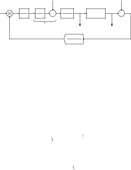
A block diagram describing the dynamics of the novel polarimeter of Figure 12.42.
The FR can be eliminated because the water solvent in the chamber has a Verdet constant and, when subject to ac and dc magnetic fields, causes optical rotation of the transmitted LPL. The glucose solute is optically active, so, in the same path length, Faraday rotation occurs because of the action of B on the water and optical rotation occurs because of the dissolved D-glucose.
It is possible to summarize the operation of this interesting system by a block diagram, shown in Figure 12.44. The input to the measurement system
© 2004 by CRC Press LLC

Examples of Special Analog Circuits and Systems |
521 |
is the physical angle of rotation of the polarization vector, φs, caused by passing the LPL through the optically active analyte. The negative feedback of the system output voltage, Vo, leads to a Faraday counter-rotation of the LPL, φF, forming a net (error) rotation, φe. The dc counter-rotation, φF, is simply:
|
|
|
|
|
φF |
= VBL′ = V(3 4) μN L′ Ic |
= [V(3 4)μN] − |
||
|
|
|
L′ |
|
VoR ˘ |
= −KFRVo (12.94) |
|
|
˙ |
|
|
||
R1RF ˚ |
|
|
Clearly, KFR = V (3/4) μ N R/(R1RF) degrees/volt. The closed-loop response of the system is found from the block diagram:
Vo |
(s) = |
|
|
|
|
−I4θmoKPKLKi (τis + 1) |
|
|
|
|
|
|
(12.95) |
||||||||||
|
2 |
τ |
|
+ s 1+ τ I |
θ |
|
K |
K |
K |
K |
FR ] |
+ I |
θ |
|
K |
K |
K |
K |
|
||||
φ |
s |
s |
L |
mo |
mo |
FR |
|||||||||||||||||
|
|
|
[ |
i 4 |
|
P |
L |
i |
|
4 |
|
P |
L |
i |
|
||||||||
It is of interest to consider the dc or steady-state response of this closedloop polarimeter to a constant φs. This can be shown to be:
Vo |
= |
−1 |
(12.96) |
||
|
|
||||
φ |
s |
|
K |
FR |
|
|
|
|
|
||
Equation 12.96 is a rather serendipitous result, revealing that the system’s calibration depends only on KFR, which depends on the transconductance of the VCCS, the dimensions and number of turns of the coil, the Verdet constant, and the permeability (μ) of water. The dc gain is independent of the light intensity (I4), the depth of polarization angle modulation (θmo), the frequency of modulation (ωm), and the system’s gain parameters (KP, KL, and Ki) and time constants (τL and τi ).
The prototype system built and tested by Browne et al. (1997) was evaluated for D-glucose concentrations (x) from 60 to 140 mg/dl. By least meansquare error curve fitting, the output voltage (y) was found to follow the linear model,
y = 0.0544 x + 0.0846 |
(12.97) |
with R2 = 0.9986. System resolution was 10.1 μo/mV out, at 27∞C with a 10-cm cell, and the glucose sensitivity was 55.4 mV/mg%. Noise in Vo was reduced by low-pass filtering (not shown in Figure 12.42).
Note that, in this instrument, op amps were used exclusively for all active components, including the photodiode current-to-voltage converter (transresistor) (see Section 2.6.4 in Chapter 2); the phase-sensitive rectifier (see Section 12.2.3 in Chapter 12); the low-pass filter (see Section 7.2 in Chapter 7); the PI integrator (see Section 6.6 in Chapter 6); the oscillator (see Section 5.5 in Chapter 5); and the VCCS (see Section 4.4 in Chapter 4).
© 2004 by CRC Press LLC

522 |
Analysis and Application of Analog Electronic Circuits |
12.8.3A Laser Velocimeter and Rangefinder
Many conventional laser-based velocimeters are based on a time-of-flight rangefinder principle in which laser pulses are reflected from a reflective (cooperative) target back to the source position and the range is found from the simple relation:
L = c t 2 meters |
(12.98) |
If the target is moving toward or away from the laser/photosensor assem-
·
bly, the relative velocity can be found by approximating v = L by numerically differentiating the sequence of return times for sequential output pulses, Dt = tk. In 1992, Laser Atlanta made a vehicular velocimeter that used this principle.
The laser velocimeter and rangefinder (LAVERA) system described in this section uses quite a different principle to provide simultaneous velocity and range output. The LAVERA system was developed by Northrop (1997) and reduced to practice by a graduate student (Nelson, 1999) for his MS research in biomedical engineering at the University of Connecticut. The motivation for developing the system was to make a walking aid for the blind that could be incorporated into a cane.
The system uses sinusoidally amplitude-modulated CW light from an NIR laser diode (LAD). The beam from the LAD is reflected from the target object and then travels back to the receiver photosensor where its intensity is converted to an ac signal whose phase lags that of the transmitted light. The phase lag is easily seen to be:
φ = (2π)( t T) = (2π)(2L c) T radians |
(12.99) |
where, as discussed previously, t is the time it takes a photon to make a round trip to the target; T is the period of the modulation; and c is the speed of light.
The system developed is a closed-loop system that tries to keep Δφ constant regardless of the target range, L. This means that, as L decreases, T must decrease and, conversely, as L increases, T must increase to maintain a constant phase difference. Figure 12.45 illustrates the functional architecture of the LAVERA system. Start the analysis by considering the voltage-to- period converter (VPC), which is an oscillator in which the output period is
proportional to VP. Thus: |
|
T = 1/f = KVPC VP + b seconds |
(12.100) |
By way of contrast, the output from a conventional voltage-to-frequency oscillator is described by:
f = KVCO VC + d Hz |
(12.101) |
© 2004 by CRC Press LLC

Examples of Special Analog Circuits and Systems |
523 |
|
|
|
AMP |
PD |
FSM |
|
|
|
|
||
Vv |
|
VL |
|
|
|
|
|
Vr |
|
|
|
|
Integrator |
− |
|
−15 V |
Reference |
|
|
|
|
||
|
−Ki (τi s + 1) |
VP |
|
beam |
|
|
|
|
|||
|
|
VPC |
VCCS |
|
|
|
s |
|
|
||
|
|
|
|
|
|
HSM |
|
LAD |
L |
Target |
|
CMP05
L
Vφ |
dc offset |
P |
AMP |
PD |
Target |
|
& LPF |
Q |
|
|
beam |
|
|
|
|
|
|
|
|
EOR |
|
|
|
−15 V
CMP05
FIGURE 12.45
Block diagram of the LAVERA system developed by Nelson (1999). Sinusoidal modulation of the laser beam’s intensity was used because less bandwidth is required for signal conditioning than for a pulsed system. The system simultaneously measures target range and velocity.
P
Q
R |
R |
|
|
|
R |
|
|
LPF |
__ |
|
Vz |
|
|
|
−1.7 V |
1 |
|
Vz |
|
|
|
|
||
|
|
|
|
f |
__
 Vz
Vz
1.7 V
π/2 |
π |
3π/2 |
2π |
5π/2 |
3π |
7π/2 |
θ |
0 |
|
|
|
|
|||
|
|
|
|
|
|
|
−1.7 V
FIGURE 12.46
The EOR phase detector used in the LAVERA system, and its transfer function.
Next, consider the phase detector. This subsystem measures the phase difference between the transmitted modulated signal intensity and the delayed, reflected modulated signal intensity. An analog multiplier can be used directly to measure this phase difference; however, in this system, the analog sine waves proportional to light intensity are passed through comparators to convert them to TTL waves with a phase difference sensed by
© 2004 by CRC Press LLC

524 |
Analysis and Application of Analog Electronic Circuits |
an exclusive or (EOR) gate phase detector (PD). The EOR PD is a quadrature detector, i.e., its output duty cycle is 50% when one input lags (or leads) the other by odd multiples of π/2. Figure 12.46 (adapted from Northrop, 1990) illustrates the EOR PD’s waveforms and transfer function. The op amp
inverts the TTL output of the EOR gate and subtracts a dc level so that Vz swings ±1.7 V.
For a heuristic view of how the system works, the PD output can be written as:
Vφ = |
|
= Vv = −(3.4 π)φ + 1.7 volts |
(12.102) |
Vz |
In the steady-state with fixed L, Vv = 0 in a type 1 feedback loop. For Vv = 0, φss = π/2. However, it has already been established that the phase lag for a returning modulated light beam is:
φ = |
( |
2π |
)( |
)( |
) |
|
(12.103) |
|
|
2 L c 1 T |
|
radians |
If Equation 12.103 for φ is solved for T and T is substituted into the VPC equation,
Tss = (2π)(2 L c)(1 φss ) = KVPC VPss + b |
(12.104) |
¬ |
|
8 L c = KVPC [VLss − Vr ]+ b |
(12.105) |
If Vr ∫ b/KVPC, the final expression for VLss is obtained: |
|
VLss = 8 L (c KVPC ) |
(12.106) |
The steady-state VL is indeed proportional to L. Going back to the VPC equation, one finds that, for a stationary target, the steady-state VPC output frequency is given by:
fss = 1 Tss = c (8L) Hz. |
(12.107) |
At L = 1m, fss = 37.5 MHz; when L = 30 m, fss = 1.25 MHz, etc.
Now suppose the target is moving away from the transmitter/receiver at
·
a constant velocity, v = L. Vv is no longer zero, but can be found from the integrator relation:
˙ |
|
˙ |
|
|
|
−8L |
|
||
Vv = −VL |
Ki = |
|
(12.108) |
|
Ki KVPC c |
||||
|
|
|
© 2004 by CRC Press LLC
Examples of Special Analog Circuits and Systems |
525 |
|
|
|
|
1.7 V |
|
|
Vr |
|
|
|
|
|
|
LPF |
|
Integrator |
− |
|
|
L |
4π |
φ |
−3.4 |
1 |
Vφ |
−Ki (τis + 1) |
VP |
||
|
|||||||||
|
c |
|
π |
(τls + 1) |
|
s |
|
|
|
|
f |
|
|
|
|
|
|
|
|
|
|
|
EOR PD |
|
|
|
|
|
|
|
|
|
|
|
Vv |
|
VL |
|
|
|
|
|
|
VPC |
|
|
|
|
|
|
|
|
|
1 |
|
|
|
|
|
|
|
|
|
KVPCVP + b |
|
|
|
||
FIGURE 12.47
Systems block diagram of the LAVERA system of Figure 12.45.
Notice the sign of Vv is negative for a receding target; also, as the target recedes, the VPC output frequency drops. Clearly, practical considerations set a maximum and a minimum for L. The limit for near L is the upper modulation frequency possible in the system; the limit for far L is the diminishing intensity of the return signal, and noise.
To appreciate the closed-loop dynamics of the LAVERA system, it is possible to make a systems block diagram as shown in Figure 12.47. Note that this system is nonlinear in its closed-loop dynamics. It can be shown (Nelson, 1999) that the closed-loop system’s undamped natural frequency, ωn, and damping factor are range dependent, even though the steady-state range and velocity sensitivities are independent of L. The undamped natural frequency for the LAVERA system of Figure 12.47 can be shown to be:
ω |
n |
= |
4(3.4)c Ki KVPC |
r s |
(12.109) |
||
|
|||||||
|
64 |
τi |
Lo |
|
|
||
|
|
|
|
||||
The closed-loop LAVERA system’s damping factor can be shown to be:
|
1 |
|
64 L |
|
˘ |
4(4.3)c K |
i |
K |
VPC |
|
ξ = |
|
o |
+ τi ˙ |
|
|
(12.110) |
||||
2 |
4(3.4)c K |
K |
64 τ L |
|
|
|||||
|
|
|
|
i VPC |
˚ |
i o |
|
|
||
Finally, to illustrate the ubiquity of the op amp in electronic instrumentation, refer to Figure 12.48 — the complete prototype LAVERA system built by Nelson (1999). Op amp subsystems will be discussed, beginning clockwise with the voltage-controlled current source (VCCS). The VCCS is used to drive the laser diode with a current of the form:
iLD(t) = ILDo + IDm sin(ωt), ILDo > IDm. |
(12.111) |
© 2004 by CRC Press LLC

+0.05 V
|
|
VR |
1N4148 |
|
VFC |
|
|
|
|
Vf |
1V pk sinewave v1 |
||||
|
1k |
|
|
|
|||
|
vi’ |
|
|
|
MAX038 |
|
|
|
|
|
|
|
|
|
|
|
|
1k |
|
|
|
|
|
|
|
|
VPVf /10 |
|
VP |
|
|
|
|
|
|
|
|
Vz = 7.9V |
−5 V |
−15 V |
|
|
|
AD532 AM |
|
||
|
|
|
1k |
|
|||
|
|
|
|
|
|
|
|
50k |
|
10k |
|
500 |
0.1 μF |
1N4148 |
|
|
|
|
|
|
|
|
|
10k |
|
|
|
|
|
1k |
|
|
|
|
500 |
|
|
|
|
|
|
|
Vv |
|
|
VL |
10k |
|
|
|
|
|
|
||
|
10k |
1k |
|
|
|
|
|
|
|
|
|
|
Ref. Sig. |
|
AD829 |
|
|
|
|
|
CMP05 |
|
|
|
|
|
|
|
|
|
|
|
|
|
10k |
|
|
90 pF |
|
|
|
|
|
|
|
|
|
|
4.7 μF |
LPF |
74F86 |
|
|
|
|
|
|
|
|
Rcvd. Sig. |
CMP05 |
AD829 |
|
|
|
|
|
|
|
|
|
|
|
|
|
|
|
90 pF |
|
|
|
|
|
|
|
cable |
|
10k
LM6313
2k 
1k
2k |
1k |
1k
LM6313
0.047 μF
100
3.3k
3.3k
100
0.047 μF
FIGURE 12.48
Simplified schematic of the LAVERA system showing the ubiquitous use of op amps.
110 Ω
RF
VCCS
1k
|
LM6313 |
−vD |
|
|
ZD |
|
iLD |
|
100k |
|
|
|
NDF |
CQL800 |
|
|
LAD |
|
PD |
OBJ |
AD829 |
|
|
|
|
−15 V
100k
PD
AD829
−15 V
526
Circuits Electronic Analog of Application and Analysis
© 2004 by CRC Press LLC
Examples of Special Analog Circuits and Systems |
527 |
This 3-op amp circuit was analyzed in detail in Section 4.4 in Chapter 4. At mid-frequencies, it was shown that iLD(t) = −v1(t) GM = −v1(t)/110 amps. The zener diode is to protect the LAD from excess forward or reverse voltage.
A Philips CQL800, 675-nm, 5-mW laser diode (LAD) was used. A small fraction of its modulated light was directed in a very short path (approximately 1 cm) through a neutral density filter (NDF) to the reference photodiode (PD). The PDs were Hammamatsu S2506-02 PIN photodiodes with spectral response from 320 to 1100 nm, with a peak at 960 nm. PD responsivity was approximately 0.4 A/W at 660 nm. The reference and received signal channels were made identical to avoid phase bias between channels; the receiver PD viewed the target through a collimated, inexpensive telescope. The photocurrents from the PDs were proportional to the light intensities striking their active areas and amplified by AD829 high-frequency op amp transresistors.
The AD829 has an fT = 120 MHz, a slew rate of η = 230 V/μs, and ena = 2 nV/ Hz. The voltage outputs from the AD829 transresistors were passed
through a simple R–C high-pass filter to block dc. The HPF corner frequencies were 10 kHz. The high-pass filtered signals were then amplified by AD829 inverting amplifiers with gains of −100. A 90-pF capacitance to ground was placed at the input of the reference channel comparator to compensate for the measured 90-pF capacitance of the shielded cable coupling the receiver channel AD829 to its comparator. PMI CMP05 amplitude comparators were used to convert the sinusoidal signals at the outputs of the AD829 amplifiers to TTL digital signals, which were then input to the exclusive OR gate used as a quadrature phase detector. The EOR output was low-pass filtered, and amplified; then a negative voltage of approximately 1.7 V was added to make Vv = 0 when the phase difference was 90∞ between the reference and received channels (see Figure 12.46).
The nearly dc Vv is then integrated by the PI integrator. (The zero from
the PI integrator is required for good closed-loop LAVERA system dynamic
·
response.) As shown previously, Vv is proportional to target velocity, L. The integrator output, VL, is proportional to target range L. VL is conditioned by a precision half-wave rectifier circuit to prevent the input to the VPC circuit from going negative, which locks up the system. The 7.9 V zener is also used to limit the input to the VPC, VP.
The voltage-to-period converter (VPC) uses a Maxim MAX038 wide-range VFC that has a 0.1-Hz to 20-MHz operating range and a sinusoidal output. A nonlinear op amp circuit is used to convert VP to Vf so that VP v1 has an over-all VPC characteristic. To examine how the nonlinear circuit works, assume the op amp is ideal and write a node equation on its summing junction (note that Vi′ = VR):
VR G + (VR − VP Vf 10)G = 0 |
(12.112) |
¬ |
|
2VR = VPVf 10 |
(12.113) |
© 2004 by CRC Press LLC
528 |
Analysis and Application of Analog Electronic Circuits |
|
If VR = 1/20 = 0.05 V, then it is clear that |
|
|
|
Vf = 1/VP |
(12.114) |
The VFC output frequency is approximately |
|
|
|
f = Kf Vf = Kf VP Hz |
(12.115) |
or |
|
|
|
T = 1/f = VP Kf = KVPC VP |
(12.116) |
The sinusoidal output of the MAX038 VFC, v1, is a 1-V peak sine wave that is used to drive the LAD.
Nelson (1999) reported a prototype CW LAVERA system with a linear VL
vs. L characteristic over 1 m ≤ L ≤ 5 m range with an R2 = 0.998. A linear Vv
·
vs. L was observed over 0.5 to 2 m/s. Wider dynamic ranges were limited by practical considerations, not by the circuit.
A problem to be solved in order to develop a practical system is how to use the velocity and range output voltages from the system to generate an audible or tactile signal that can warn a blind person of moving objects that may present a hazard. Vv goes positive for a moving target approaching the system, negative for a receding target, and zero for a stationary target. Thus, Vv might be used to control the pitch of an audio oscillator (not shown) around some zero-velocity frequency, e.g., 550 Hz. An approaching target would raise the audio pitch to as high as 10 kHZ; a receding target might lower the velocity pitch to 30 Hz minimum. But how is the range coded? Range is always positive and close objects should demand more attention, so another VPC circuit (not shown) can be used to generate “click” pulses that can be added to the velocity tone signal. Thus, a rapidly approaching constant velocity vehicle would generate a high, steady sinusoidal tone plus a click rate of increasing frequency as the range decreases. If the vehicle stops nearby, e.g., at a traffic light, the sinusoidal tone would drop to the 0-V frequency (550 Hz), but the click rate would remain high, e.g., 20/sec for a 2-m L.
12.8.4Self-Balancing Impedance Plethysmographs
One way to measure the volume changes in body tissues is by measuring the electrical impedance of the body part being studied. As blood is forced through arteries, veins, and capillaries by the heart, the impedance is modulated. When used in conjunction with an external air pressure cuff that can gradually constrict blood flow, impedance plethysmography (IP) can provide noninvasive diagnostic signs about abnormal venous and arterial blood
© 2004 by CRC Press LLC

Examples of Special Analog Circuits and Systems |
529 |
flow. Also, by measuring the impedance of the chest, the relative depth and rate of a patient’s breathing can be monitored noninvasively. As the lungs inflate and the chest expands, the impedance magnitude of the chest increases; air is clearly a poorer conductor than tissues and blood.
For safety’s sake, IP is carried out using a controlled ac current source of fixed frequency. The peak current is generally kept less than 1 mA and the frequency used typically is between 30 to 75 kHz. The high frequency is used because human susceptibility to electroshock, as well as physiological effects on nerves and muscles from ac, decreases with increasing frequency (Webster, 1992). The electrical impedance can be measured indirectly by measuring the ac voltage between two skin surface electrodes (generally ECGor EEG-type, AgCl + conductive gel) placed between the two current electrodes. Thus, four electrodes are generally used, although the same two electrodes used for current injection can also be connected to the high-input impedance, ac differential amplifier that measures the output voltage, Vo. By Ohm’s law, the body voltage is: Vo = Is Zt = Is [Rt + j Bt].
At a fixed frequency, the tissue impedance can be modeled by a single conductance in parallel with a capacitor; thus, it is algebraically simpler to consider the tissue admittance, Yt = Zt−1 = Gt + jωCt. Gt and Ct change as blood periodically flows into the tissue under measurement. The imposed ac current is carried in the tissue by moving ions, rather than electrons. Ions such as Cl−, HCO3−, K+, Na+, etc. drift in the applied electric field (caused by the current-regulated source); they have three major pathways: (1) a resistive path in the extracellular fluid electrolyte; (2) a resistive path in blood; and
(3) a capacitive path caused by ions that charge the membranes of closely packed body cells.
Ions can penetrate cell membranes and move inside cells, but not with the ease with which they can travel in extracellular fluid space and in blood. Of course, many, many cells are effectively in series and parallel between the current electrodes. Ct represents the net equivalent capacitance of all the cell membranes. Each species of ion in solution has a different mobility. The mobility of an ion in solution is μ ∫ v/E, where v is the mean drift velocity of the ion in a surrounding uniform electric field, E. Ionic mobility also depends on the ionic concentration, as well as the other ions in solution. Ionic mobility has the units of m2 sec−1 V−1. Returning to Ohm’s law, one can write in phasor notation:
Vo = Is Yt = Is |
Gt |
− jωCt |
= Is [Re{Zt}− j Im{Zt}] |
(12.117) |
G 2 |
+ ω2C 2 |
|||
|
t |
t |
|
|
where Re{Zt} = Gt/(Gt2 + ω2Ct2) is the real part of the tissue impedance and Im{Zt} = Bt = −ωCt (Gt2 + ω2Ct2) is the imaginary part of the tissue impedance.
Note that Re{Zt} and Im{Zt} are frequency dependent and that Vo lags Is. There are several ways of measuring tissue Zt magnitude and angle. In
the first method, described in detail later, an ac voltage, Vs, is applied to the
© 2004 by CRC Press LLC

530 |
Analysis and Application of Analog Electronic Circuits |
|||
|
|
|
|
Current-to- |
|
|
|
|
voltage converter |
75 MHz oscillator |
Electrodes |
Thorax |
|
|
|
|
|
CF |
|
|
|
|
|
|
|
Buffer |
|
|
|
|
Vs |
Gt |
|
RF |
|
|
|
||
HPF |
|
Ct |
Io |
|
(TTL) |
|
|
|
|
|
|
|
|
|
|
|
|
|
HPF |
|
Phase- |
|
|
|
|
shifter |
|
|
|
C |
|
|
Sync |
|
|
|
|
|
|
R |
V1 |
|
|
Vo |
|
|
Ve |
||
|
|
|
PSR |
DA |
|
LPF |
|
|
VF |
|
|
|
|
|
Integrator |
|
|
|
|
V2 |
|
Vs |
|
|
|
|
+ |
|
|
VB |
|
Vc |
|
|
+ |
|
Summer |
HPF |
|
|
FIGURE 12.49
Block diagram of the author’s self-nulling admittance plethysmograph.
tissue. The amplitude is adjusted so that the resultant current, Io, remains less than 1 mA. Io is converted to a proportional voltage, Vo, by an op amp current-to-voltage converter circuit. In general, Vo and Vs differ in phase and magnitude. A self-nulling feedback circuit operates on Vo and Vs. At null, its output voltage, Vc, is proportional to Zt .
A second method uses the ac current source excitation, Is; the output voltage described previously, Vo, is fed into a servo-tracking two-phase lockin amplifier, which produces an output voltage, Vz Zt , and another voltage, Vθ –Zt. A self-nulling plethysmograph designed by the author is illustrated in Figure 12.49. A 75-kHz sinusoidal voltage, Vs, is applied to a chest electrode. An ac current phasor, Io, flows through the chest to virtual ground and is given by Ohm’s law:
Io = Vs [Gt + jωCt] |
(12.118) |
This current is converted to ac voltage, Vo, by the current-to-voltage op amp:
© 2004 by CRC Press LLC

Examples of Special Analog Circuits and Systems
|
|
|
Vo = − |
|
|
Io |
|
|
|
|
|
|
|
|
|
|
|
GF |
+ jωCF |
|
|
|
|
||||||
|
|
|
|
|
|
|
|
|
||||||
|
|
|
|
¬ |
|
|
|
|
|
|
|
|
||
Vo = −Io |
GF − jωCF |
= −Vs[Gt |
+ jωCt ] |
GF − jωCF |
||||||||||
G 2 |
+ |
ω2C 2 |
G 2 |
+ ω2C |
2 |
|||||||||
|
F |
|
F |
|
|
|
|
|
|
F |
|
|
|
F |
|
|
|
|
¬ |
|
|
|
|
|
|
|
|
||
Vo = −Vs |
G G − jωC |
G + jωC G + ω2C C |
F |
|
||||||||||
t |
F |
|
F |
|
t |
|
t F |
t |
|
|||||
|
|
|
G 2 + ω2C 2 |
|
|
|
|
|||||||
|
|
|
|
|
|
|
F |
|
F |
|
|
|
|
|
531
(12.119)
(12.120)
(12.121)
With the patient exhaled and holding his breath, CF is adjusted so that Vo is in phase with Vs. That is, CF is set so that the imaginary terms in Equation 12.121 0. That is,
|
CF = CFo ∫ Cto |
(RFGto ). |
|
(12.122) |
|||
Then, |
|
|
|
|
|
|
|
Vo = −Vs |
G G |
F |
+ ω2C C |
Fo |
−Vs (RF |
Rto ) |
(12.123) |
to |
to |
||||||
G |
2 |
+ ω2C 2 |
|
||||
|
F |
Fo |
|
|
|
|
|
Now when the patient inhales, the lungs expand and the air displaces conductive tissue, causing the parallel conductance of the chest, Gt, to decrease from Gto. Substitute Gt = Gto + δGt and Ct = Cto + δCt into Equation 12.121 and also let RFCF = Cto Rto from the initial phase nulling. After a considerable amount of algebra,
Vo |
(jω) = |
−RF |
|
|
[Gto (1+ δGt Gω )+ ω2 |
(RFCF )2 Gto (1+ δCt Cto )+ |
|
|
|
2 |
] |
||||
Vs |
[1+ ω2 (RFCF ) |
|
|
|
|||
|
|
|
|
|
jωCto (δCt Cto − δGt Gto )] |
(12.124) |
|
This relation reduces to Equation 12.123 for δCt = δGt 0. If it is assumed that δCt 0 only, then Equation 12.124 can be written:
Vo + δVo |
δGt RF |
|
|
|
(jω) −RFGto − [1+ ω2 (RFCF )2 |
] |
(12.125A) |
Vs |
where
© 2004 by CRC Press LLC

532 |
Analysis and Application of Analog Electronic Circuits |
+ |
|
|
|
|
|
|
|
|
+ |
+ |
|
|
|
|
|
|
−Vs |
|
δGt |
|
|||||||||
|
|
|
− RF Gto |
|
|
|
|
|
|
|
|
|
|
||||||||||||||||
Vs |
|
|
|
|
|
|
|
|
|
|
|
|
|
||||||||||||||||
|
|
|
|
(ac) |
|
|
|
|
|
|
|
[1 + (ωRFCF)2 ] |
|
|
|
|
|
|
|||||||||||
|
|
|
|
|
|
|
|
|
|
|
|
|
|
|
|
|
|
|
|
|
|
|
|
|
|
|
|
|
|
(ac) |
|
|
|
|
|
|
|
Vo + δVo |
|
|
|
|
|
|
|
|
|
|
|
|
|
|
PSD |
|
|||||
|
|
|
|
|
|
|
|
|
|
|
|
|
|
|
|
|
|
|
|
|
|
||||||||
|
|
|
|
|
|
|
|
|
|
|
|
|
|
|
|
|
|
|
|
|
|
|
|
|
|||||
|
|
|
|
|
|
|
|
|
+ |
|
|
|
|
|
|
|
|
|
|
|
|
|
|
|
|||||
|
|
|
|
|
|
|
|
|
|
|
|
|
|
|
|
|
|
|
|
|
|
|
|
|
|
|
|
||
|
|
|
0.1 |
|
VsVc /10 |
|
|
|
|
|
KA |
Ve |
|
|
|
KP |
|
|
|
||||||||||
|
|
|
|
|
(ac) |
|
− |
|
|
|
|
|
(ac) |
|
|
|
|
|
|
||||||||||
|
|
|
|
|
|
|
|
|
|
|
|
|
|
|
|
|
|
|
|
|
|
|
|
||||||
|
Analog |
|
|
|
|
|
|
Difference |
|
|
|
|
|
|
|
|
|
|
|
||||||||||
|
|
|
|
|
|
|
|
|
|
|
|
|
|
|
|
|
|
|
|||||||||||
Vc |
multiplier |
|
|
|
|
|
|
|
amplifier |
|
|
|
|
|
|
|
|
|
|
|
|||||||||
(dc) |
|
|
|
|
|
|
|
|
|
|
|
|
|
|
|
|
|
|
|
|
|
|
|
|
LPF |
|
|||
|
|
|
|
|
|
|
|
|
|
|
|
|
|
|
|
|
|
|
|
|
|
|
|
|
|
|
|
|
|
|
|
|
|
|
|
|
|
+ |
|
|
|
|
(dc) |
|
|
|
−1 |
|
|
V1 |
|
1 |
|
|
|
|
|||
|
|
−1 |
|
|
|
|
β |
|
|
|
|
|
|
|
|
|
|
||||||||||||
|
|
|
|
|
+ |
|
|
|
|
|
|
|
|
s RC |
|
|
|
|
s2/ωn2 + s2ξ/ωn + 1 |
|
|
||||||||
|
|
Summer |
|
|
Loop gain |
|
|
|
|
|
|
|
|
|
|
|
|
|
|
|
|
||||||||
|
|
|
|
|
|
|
Integrator |
|
|
|
|
|
|
|
|
||||||||||||||
|
|
|
|
|
|
|
|
|
|
|
|
|
|
|
|
||||||||||||||
|
|
|
|
|
|
|
|
|
adjust |
|
|
|
|
|
|
|
|
|
|
|
|
|
|
||||||
|
|
|
|
|
|
|
|
|
|
|
|
|
|
|
|
|
|
|
|
|
|
|
|
|
|
|
|
||
|
|
|
|
|
|
VB |
|
|
|
|
|
|
|
|
|
|
|
|
|
|
|
|
|
|
|
|
|
||
|
|
|
|
|
|
|
|
|
|
V2 |
|
|
|
|
|
|
|
|
|
|
|
|
|
|
|||||
|
|
|
|
|
|
(dc) |
|
|
|
|
|
|
|
|
|
|
|
|
|
|
|
|
|
|
|||||
|
|
|
|
|
|
|
|
|
|
|
|
|
|
|
|
|
|
|
|
|
|
|
|
|
|
|
|||
FIGURE 12.50
Systems block diagram describing the dynamics of the self-nulling plethysmograph.
Vo = (−RFGto )Vs |
|
(12.125B) |
(δGt )RF |
]Vs |
|
δVo = − [1+ ω2 (RFCF )2 |
(12.125C) |
Note that δGt < 0 for an inhaled breath.
Figure 12.50 illustrates a systems block diagram for the author’s selfbalancing plethysmograph, configured for the condition where δCt 0. The three RC high-pass filters in Figure 12.49 are used to block unwanted dc components from Vs, Vo, and VF. In the first case, δGt 0. In the steady state, Ve 0, so:
VsVc 10 = −VsRFGto |
(12.126) |
Thus, |
|
Vc = −10 RFGto = −(VB + βV2 ), |
(12.127) |
and the dc integrator output, V2, is proportional to Gto: |
|
V2 = (10 RFGto − VB ) β |
(12.128) |
© 2004 by CRC Press LLC