noise (Northrop, 2002, 2003). Evoked transient electrical response can be recovered by averaging even when the input SNR to the averager is as low as −60 dB.

1.6.3Other Body Surface Potentials

The electrooculogram (EOG), electroretinogram (ERG), and electrocochleogram (ECoG) are transient, low-amplitude, low-bandwidth potentials recorded for diagnostic and research purposes (Northrop, 2002). Each transient waveform is generally accompanied by unwanted, uncorrelated noise from EMGs and from the electrodes. The EOG is the largest of these three potentials, with a peak on the order of single millivolt. Thus, an ECG amplifier can be used with a 0.05 to 100 Hz −3-dB bandwidth and gain of 103. Averaging is generally not required.

The ERG, on the other hand, has a peak amplitude on the order of hundreds of microvolts and accompanying noise makes signal averaging expeditious. The ERG preamplifier generally has a band pass of 0.3 to 300 Hz, a gain of between 103 and 104, and an input impedance of at least 10 MΩ.

The electrocochleogram is the lowest amplitude transient, with a peak of only approximately 6 μV and waveform features of <1 μV. Signal averaging must be used to resolve the ECoG evoked transient. The signal conditioning amplifier has a midband gain of 104 and −3-dB frequencies of 5 and 3 kHz. The ECoG amplifier band pass is defined by 12 dB/octave (two-pole) filters.

1.7Discussion

The preceding descriptions indicate that the frequency content of endogenous signals from the body ranges from near dc to about 3 kHz. These signals are accompanied by noise, which means that linear filtering to improve the SNRin can often help. Some signals, such as ECoG and evoked brain cortical transients, require signal averaging for meaningful resolution. Endogenous signal peak amplitudes range from over 100 mV for nerve and muscle transmembrane potentials recorded with glass micropipette electrodes to less than a microvolt for evoked cortical transients recorded on the scalp.

1.8Electrical Properties of Bioelectrodes

To record biopotentials, an interface is needed between the electron-conduct- ing copper wires connected to signal conditioning amplifiers and the ion-conducting, “wet” environment of living animals. Electrodes form this

© 2004 by CRC Press LLC

interface. Some of the many kinds of electrodes are better than others in terms of low noise and ease of use. Early ECG electrodes were nondisposable, nickel–silver-plated copper, or stainless steel disks hard-wired to the amplifier input leads. Although conductive gel was used, this type of electrode had inherently high low-frequency noise due to the complex redox reactions taking place at the metal electrode surfaces. Still, acceptable ECG and EMG signals could be recorded.

Present practice in measuring ECG and EMG signals from the skin surface is to use disposable sticky patch electrodes. Patch electrodes use a silverΩsilver chloride interface to a conductive gel containing Na+, K+, and Cl– ions. The gel makes direct, wet contact with the skin. Adhesive for the skin is found in a ring surrounding the electrolyte and AgCl. The copper wire makes contact with the Ag metal backing of the electrode, generally with a snap connector. More recently, skin electrodes have used AgΩAgCl deposited in a thin layer on an approximately 2.5-cm square of thin plastic film. The conductive gel and adhesive are combined in a layer all over the AgCl film. Contact with this inexpensive electrode is made with a miniature metal alligator clip on one raised corner.

Silver chloride is used with skin patch electrodes and many other types because the dc half-cell potential of the AgΩAgCl electrode depends on the logarithm of the concentration of chloride ions (Webster, 1992). Because the AgCl is in direct contact with the coupling gel, which has a high concentration of Cl− ions, the dc half-cell potential of the electrode remains fairly stable and has a low impedance, thus low thermal noise.

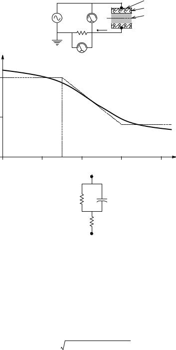
Figure 1.5 illustrates the electrical characteristics of a pair of AgΩAgCl electrodes facing each other. The impedance measured as a function of frequency, Ω2 Zel(f) Ω suggests that each electrode can be modeled by a parallel R–C circuit in series with a resistance. Analysis of the impedance magnitude in this figure reveals that RG = 65 Ω, Ri = 1935 Ω, and Ci = 0.274 μF for one electrode. The skin also adds a parallel R–C circuit to the electrode’s equivalent circuit.

In general, it is desirable for the electrode Z to be as small as possible. Both resistors in the electrode model make thermal (white) noise. At low frequencies

where the capacitive reactance is 1935 Ω, one electrode’s root noise spectrum is 4kT 2000 = 5.76 nV RMS/ Hz — the same order of magnitude as an

amplifier’s equivalent short-circuit input noise. If the gel dries out during prolonged use, the Zel will rise, as will the white noise from its real part.

Another type of electrode used in neurophysiological research is the salinefilled, glass micropipette electrode used for recording transmembrane potentials in neurons and muscle fibers. Because the tips of these electrodes are drawn down to diameters of a fraction of a micron before filling, their resistances when filled can range from approximately 20 to 103 MΩ, depending on the tip geometry, the filling medium, and the surround medium in which the tip is placed. Because of their high series resistances, glass micropipette electrodes create three major problems not seen with other types of bioelectrodes:

© 2004 by CRC Press LLC

1Ω Ie

(2 electrodes)

AC equivalent circuit for one electrode

C

RG

FIGURE 1.5

(A) Impedance magnitude measurement circuit for a pair of face-to-face, silver–silver chloride skin surface electrodes. (B) Typical impedance magnitude for the pair of electrodes in series. (C) Linear equivalent circuit for one electrode.

1.Because of their high series resistances, they must be used with special signal conditioning amplifiers called electrometer amplifiers,

which have ultra-low, input dc bias currents. Electrometer input bias currents are on the order of 10 fA (10−14 A) and their input resistances are approximately 1015 Ω.

2.Glass micropipette electrodes make an awesome amount of Johnson noise. For example, a 200 MΩ electrode at 300 K, with a noise band-

width of 3 kHz, makes 4kT ∞ 2 ∞ 108 ∞ 3 ∞ 103 = 99.68 μV RMS of noise.

© 2004 by CRC Press LLC

CN

E

Vo

EA

Filling electrolyte

AgCl electrode

Extracellular electrolyte

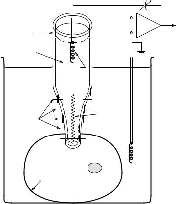
FIGURE 1.6

Schematic cross section (not to scale) of an electrolyte-filled, glass micropipette electrode inserted into the cytoplasm of a cell. AgΩAgCl electrodes are used to interface recording wires (generally Cu) with the electrolytes.

3.The tips of glass micropipette electrodes have significant distributed capacitance between the electrolyte inside and the electrolyte outside the tip (see Figure 1.6), which makes them behave like distributedparameter low-pass filters, as shown in Figure 1.7(A).

This figure also illustrates the equivalent circuits of the AgΩAgCl coupling electrodes, the cell membrane, and the microelectrode tip spreading resistance and tip EMF. The distributed resistance of the internal electrolyte in the tip, Rtip, plus the tip spreading resistance, Rtc, plus the cell membrane’s resistance, 1/Gc, are orders of magnitude larger than the impedances associated with the AgCl coupling electrodes. Thus, they can be lumped together as a single Rμ and the distributed tip capacitance can be represented by a

single, lumped Cμ in the simplified R–C LPF of Figure 1.7(B). Vbio is the bioelectric EMF across the cell membrane in the vicinity of the microelectrode tip. The break frequency of the B circuit is simply fb = 1/(2πRμCμ) Hz.

© 2004 by CRC Press LLC