

- •Analysis and Application of Analog Electronic Circuits to Biomedical Instrumentation
- •Dedication
- •Preface
- •Reader Background
- •Rationale
- •Description of the Chapters
- •Features
- •The Author
- •Table of Contents
- •1.1 Introduction
- •1.2 Sources of Endogenous Bioelectric Signals
- •1.3 Nerve Action Potentials
- •1.4 Muscle Action Potentials
- •1.4.1 Introduction
- •1.4.2 The Origin of EMGs
- •1.5 The Electrocardiogram
- •1.5.1 Introduction
- •1.6 Other Biopotentials
- •1.6.1 Introduction
- •1.6.2 EEGs
- •1.6.3 Other Body Surface Potentials
- •1.7 Discussion
- •1.8 Electrical Properties of Bioelectrodes
- •1.9 Exogenous Bioelectric Signals
- •1.10 Chapter Summary
- •2.1 Introduction
- •2.2.1 Introduction
- •2.2.4 Schottky Diodes
- •2.3.1 Introduction
- •2.4.1 Introduction
- •2.5.1 Introduction
- •2.5.5 Broadbanding Strategies
- •2.6 Photons, Photodiodes, Photoconductors, LEDs, and Laser Diodes
- •2.6.1 Introduction
- •2.6.2 PIN Photodiodes
- •2.6.3 Avalanche Photodiodes
- •2.6.4 Signal Conditioning Circuits for Photodiodes
- •2.6.5 Photoconductors
- •2.6.6 LEDs
- •2.6.7 Laser Diodes
- •2.7 Chapter Summary
- •Home Problems
- •3.1 Introduction
- •3.2 DA Circuit Architecture
- •3.4 CM and DM Gain of Simple DA Stages at High Frequencies
- •3.4.1 Introduction
- •3.5 Input Resistance of Simple Transistor DAs
- •3.7 How Op Amps Can Be Used To Make DAs for Medical Applications
- •3.7.1 Introduction
- •3.8 Chapter Summary
- •Home Problems
- •4.1 Introduction
- •4.3 Some Effects of Negative Voltage Feedback
- •4.3.1 Reduction of Output Resistance
- •4.3.2 Reduction of Total Harmonic Distortion
- •4.3.4 Decrease in Gain Sensitivity
- •4.4 Effects of Negative Current Feedback
- •4.5 Positive Voltage Feedback
- •4.5.1 Introduction
- •4.6 Chapter Summary
- •Home Problems
- •5.1 Introduction
- •5.2.1 Introduction
- •5.2.2 Bode Plots
- •5.5.1 Introduction
- •5.5.3 The Wien Bridge Oscillator
- •5.6 Chapter Summary
- •Home Problems
- •6.1 Ideal Op Amps
- •6.1.1 Introduction
- •6.1.2 Properties of Ideal OP Amps
- •6.1.3 Some Examples of OP Amp Circuits Analyzed Using IOAs
- •6.2 Practical Op Amps
- •6.2.1 Introduction
- •6.2.2 Functional Categories of Real Op Amps
- •6.3.1 The GBWP of an Inverting Summer
- •6.4.3 Limitations of CFOAs
- •6.5 Voltage Comparators
- •6.5.1 Introduction
- •6.5.2. Applications of Voltage Comparators
- •6.5.3 Discussion
- •6.6 Some Applications of Op Amps in Biomedicine
- •6.6.1 Introduction
- •6.6.2 Analog Integrators and Differentiators
- •6.7 Chapter Summary
- •Home Problems
- •7.1 Introduction
- •7.2 Types of Analog Active Filters
- •7.2.1 Introduction
- •7.2.3 Biquad Active Filters
- •7.2.4 Generalized Impedance Converter AFs
- •7.3 Electronically Tunable AFs
- •7.3.1 Introduction
- •7.3.3 Use of Digitally Controlled Potentiometers To Tune a Sallen and Key LPF
- •7.5 Chapter Summary
- •7.5.1 Active Filters
- •7.5.2 Choice of AF Components
- •Home Problems
- •8.1 Introduction
- •8.2 Instrumentation Amps
- •8.3 Medical Isolation Amps
- •8.3.1 Introduction
- •8.3.3 A Prototype Magnetic IsoA
- •8.4.1 Introduction
- •8.6 Chapter Summary
- •9.1 Introduction
- •9.2 Descriptors of Random Noise in Biomedical Measurement Systems
- •9.2.1 Introduction
- •9.2.2 The Probability Density Function
- •9.2.3 The Power Density Spectrum
- •9.2.4 Sources of Random Noise in Signal Conditioning Systems
- •9.2.4.1 Noise from Resistors
- •9.2.4.3 Noise in JFETs
- •9.2.4.4 Noise in BJTs
- •9.3 Propagation of Noise through LTI Filters
- •9.4.2 Spot Noise Factor and Figure
- •9.5.1 Introduction
- •9.6.1 Introduction
- •9.7 Effect of Feedback on Noise
- •9.7.1 Introduction
- •9.8.1 Introduction
- •9.8.2 Calculation of the Minimum Resolvable AC Input Voltage to a Noisy Op Amp
- •9.8.5.1 Introduction
- •9.8.5.2 Bridge Sensitivity Calculations
- •9.8.7.1 Introduction
- •9.8.7.2 Analysis of SNR Improvement by Averaging
- •9.8.7.3 Discussion
- •9.10.1 Introduction
- •9.11 Chapter Summary
- •Home Problems
- •10.1 Introduction
- •10.2 Aliasing and the Sampling Theorem
- •10.2.1 Introduction
- •10.2.2 The Sampling Theorem
- •10.3 Digital-to-Analog Converters (DACs)
- •10.3.1 Introduction
- •10.3.2 DAC Designs
- •10.3.3 Static and Dynamic Characteristics of DACs
- •10.4 Hold Circuits
- •10.5 Analog-to-Digital Converters (ADCs)
- •10.5.1 Introduction
- •10.5.2 The Tracking (Servo) ADC
- •10.5.3 The Successive Approximation ADC
- •10.5.4 Integrating Converters
- •10.5.5 Flash Converters
- •10.6 Quantization Noise
- •10.7 Chapter Summary
- •Home Problems
- •11.1 Introduction
- •11.2 Modulation of a Sinusoidal Carrier Viewed in the Frequency Domain
- •11.3 Implementation of AM
- •11.3.1 Introduction
- •11.3.2 Some Amplitude Modulation Circuits
- •11.4 Generation of Phase and Frequency Modulation
- •11.4.1 Introduction
- •11.4.3 Integral Pulse Frequency Modulation as a Means of Frequency Modulation
- •11.5 Demodulation of Modulated Sinusoidal Carriers
- •11.5.1 Introduction
- •11.5.2 Detection of AM
- •11.5.3 Detection of FM Signals
- •11.5.4 Demodulation of DSBSCM Signals
- •11.6 Modulation and Demodulation of Digital Carriers
- •11.6.1 Introduction
- •11.6.2 Delta Modulation
- •11.7 Chapter Summary
- •Home Problems
- •12.1 Introduction
- •12.2.1 Introduction
- •12.2.2 The Analog Multiplier/LPF PSR
- •12.2.3 The Switched Op Amp PSR
- •12.2.4 The Chopper PSR
- •12.2.5 The Balanced Diode Bridge PSR
- •12.3 Phase Detectors
- •12.3.1 Introduction
- •12.3.2 The Analog Multiplier Phase Detector
- •12.3.3 Digital Phase Detectors
- •12.4 Voltage and Current-Controlled Oscillators
- •12.4.1 Introduction
- •12.4.2 An Analog VCO
- •12.4.3 Switched Integrating Capacitor VCOs
- •12.4.6 Summary
- •12.5 Phase-Locked Loops
- •12.5.1 Introduction
- •12.5.2 PLL Components
- •12.5.3 PLL Applications in Biomedicine
- •12.5.4 Discussion
- •12.6 True RMS Converters
- •12.6.1 Introduction
- •12.6.2 True RMS Circuits
- •12.7 IC Thermometers
- •12.7.1 Introduction
- •12.7.2 IC Temperature Transducers
- •12.8 Instrumentation Systems
- •12.8.1 Introduction
- •12.8.5 Respiratory Acoustic Impedance Measurement System
- •12.9 Chapter Summary
- •References

5
Feedback, Frequency Response,
and Amplifier Stability
5.1Introduction
This chapter explains the details of how feedback changes open-loop amplifier frequency response and examines how NVF and PVF can lead to amplifier instability. Practical use can be made of instability; tunable sinusoidal oscillators can be designed using the same analytical techniques used in the design of linear feedback amplifiers.
Over the years, many analytical techniques have been used to analyze and design feedback systems. In the author’s opinion, the root-locus technique is one of the more useful ones. It allows the s-plane location of the closedloop (CL) system’s poles to be found, given the system’s dc or mid-frequency loop gain and the location of the poles and zeros of the system’s loop gain, AL(s). Once the closed-loop poles and zeros are known, it is a simple matter to find the CL system’s frequency response or its output in time, given a transient input.
5.2Review of Amplifier Frequency Response
5.2.1Introduction
The steady-state sinusoidal frequency response has long been a performance criterion for linear signal conditioning systems. For example, an amplifier is given a continuous sinusoidal input of known frequency and an amplitude that does not saturate the amplifier. At the output, a sinusoidal output of the same frequency, but generally with a different amplitude from the input, and a phase shifted from the input sinusoid can be measured. The amplitude and phase shift of the output are frequency dependent. The frequency response measured experimentally can be used to define the frequency response function of the amplifier. This is the 2-D vector, H(jω). In polar form:
199
© 2004 by CRC Press LLC

200 |
Analysis and Application of Analog Electronic Circuits |
|||||
|
H(jω) = |
|
Vo |
|
(ω)–θ(ω) |
(5.1) |
|
|
|
||||
|
|
V |
|
|||
|
|
|
|
|
|
|
|
|
|
s |
|
|
|
The frequency-dependent ratio of output voltage to input voltage magnitudes is called the amplitude response (AR); θ(ω) is the phase angle between the output and the input sine waves. The frequency response junction, H(ω), whether measured or calculated, is in general a 2-D vector. (It has a magnitude and an angle as shown in Equation 5.1 or, equivalently, a real and an imaginary part.)
The two major ways to present frequency response data are (1) by Bode plot and (2) by polar (Nyquist) plot. Bode plots are much more widely used to characterize analog electronic signal conditioning systems used in biomedicine, and will be considered here. Bode and Nyquist plots are considered in detail in Section 2.4 of Northrop (2003).
5.2.2Bode Plots
A Bode plot is a system’s frequency response plot done on log-linear graph paper. The (horizontal) frequency axis is logarithmic; on the linear vertical axis is plotted 20 log10 H( f ) , which has the units of decibels (dB) and the phase angle of H( f ) (the phase angle between the output and input sinusoids). One advantage of plotting 20 log10 H( f ) vs. f on semilog paper is that plots are made easier by the use of asymptotes giving the frequency response behavior relative to the system’s break or natural frequencies. Also, using a logarithmic function causes products of terms to appear graphically as sums. Perhaps the best way to introduce the art of Bode plotting is by example.
Example 1: a simple low-pass system. Assume a system is described by the first-order frequency response function:
Y |
(jω) = |
c |
= H(ω) |
(5.2) |
U |
|
|||
|
a jω + b |
|
||
It is algebraically more convenient when creating a Bode plot to have the frequency response function in time-constant form. That is, the 0th power of (s = jω) is given a coefficient of 1 in numerator and denominator, e.g.,
Y |
(jω) = |
c b |
= H(jω) (time-constant form) |
(5.3) |
|
U |
jω(a b)+ 1 |
|
|||
The quantity (a/b) is the system’s time constant, which has the units of time. One advantage of the time-constant format is that, when u is dc, ω = 0, and the dc gain of the system is simply Kvo = (c/b). The vector magnitude of the frequency response vector function is:
© 2004 by CRC Press LLC

Feedback, Frequency Response, and Amplifier Stability |
201 |
||||||
|
H(jω) |
|
= |
|
c b |
|
(5.4) |
|
|
|
|||||
|
|
ω2 |
(a b)2 + 1 |
||||
|
|
|
|
|
|||
and its dB logarithmic value is: |
|
|
|
||||
dB = 20 log(c/b) − 10 log[ω2(a/b)2 + 1] |
(5.5) |
||||||
For ω = 0, dB = 20 log(c/b). For ω = (a/b)−1 r/s, dB = 20 log(c/b) − 10 log[2], or the dc level minus 3 dB. ωo = (a/b)−1 r/s is the system’s break frequency. For ω ≥ 10ωo, the amplitude response is given by:
dB = 20 log(c/b) − 20 log[ω] − 20 log[a/b] |
(5.6) |
From the preceding equation, it is possible to see that the asymptote has a slope of −20 dB/decade of radian frequency or, equivalently, −6 dB/octave (doubling) of frequency. The phase of this system is given by:
φ(ω) = − tan−1 (ω a/b) |
(5.7) |
The minus sign is because the complex portion of Equation 5.3 is in its denominator. Thus, the phase goes from 0∞ at ω = 0 to −90∞ as ω •. Figure 5.1 illustrates the complete Bode plot for the simple first-order, low-pass system.
Example 2: this is an underdamped second-order, low-pass system described by the frequency response vector function:
|
Y |
|
|
d |
|
B |
|
|
U |
(jω) = a(jω)2 + b(jω)+ c = |
A –φ = H(jω) |
(5.8) |
|||
|
|
|
|
|
|
Asymptotes |
|
AR (dB) |
|
|
|
|
|
|
ϕ(ω/(a/b)) |
|
|
|
|
|
|
|
0o |
20 log10(c/b) |
|
|
|
|
|
−3dB |
|
|
|
|
|
|
|
|
|
|
|
|
AR (dB) |
|
|
|
|
|
|
|
|
|
|
|
−45o |
|
|
|
ϕ(ω/(a/b)) |
|
|
−20 dB |
|
|
|
|
|
|
|
|
|
0.01 |
0.1 |
0.5 |
1.0 |
2.0 |
10 |
−90o |
|
100 |
|||||||
|
|
|
|
|
|
ω/(a/b) |
|
FIGURE 5.1
Normalized Bode plot for a one real pole low-pass filter. Asymptotes, AR, and phase are shown.
© 2004 by CRC Press LLC

202 |
Analysis and Application of Analog Electronic Circuits |
To put this frequency response function in time-constant form to facilitate Bode plotting, it is necessary to divide numerator and denominator by c:
Y |
(jω) = |
d c |
= |
|
d c |
(5.9) |
U |
(a c)(jω)2 + (b c)(jω)+ 1 |
(jω)2 |
ωn2 + (2ξ ωn )(jω)+ 1 |
The constant, c/a ∫ ωn2, is the system’s undamped natural radian frequency squared and b/c ∫ 2ξ/ωn, where ξ is the system’s damping factor. The system has complex-conjugate roots to the characteristic equation of its ODE if 0 < ξ < 1. In this second example, it will be assumed that the system is underdamped, i.e., 0 < ξ < 1. Now the Bode magnitude plot is found from:
{ |
|
|
|
|
} |
|
db = 20 log(d c)− 10 log [1− ω |
2 |
2 |
2 |
2 |
|
(5.10) |
|
ωn |
] |
+ [(2ξ ωn )ω] |
|
At dc and ω ωn and ωn/2ξ, dB 20 log(d/c). The undamped natural frequency is ωn = c/a r/s. When ω = ωn, dB = 20 log(d/c) − 20 log[(2ξ/ωn) ωn] = 20 log(d/c) − 20 log[2ξ]; when ω ωn, dB = 20 log(d/c) − 40 log[ω/ωn].
Thus, for ω = ωn and ξ < 0.5, the dB curve rises to a peak above the intersection of the asymptotes. The high-frequency asymptote has a slope of −40 dB/decade of radian frequency, or −12 dB/octave (doubling) of radian frequency. These features are shown schematically in Figure 5.2. The phase of the secondorder low-pass system can be found by inspecting the frequency response function of Equation 5.9. It is simply:
φ = − tan |
−1 |
ω(2ξ ω |
)ˆ |
|
|||||
|
|
|
|
n |
|
˜ |
(5.11) |
||
|
− ω |
2 |
|
2 |
|||||
|
|
1 |
|
ωn |
↓ |
|
|||
It can be shown (Ogata, 1970) that the magnitude of the resonant peak normalized with respect to the system’s dc gain is:
Mp |
= |
|
H(jω) |
|
max |
= |
|
1 |
|
for 0.707 |
≥ ξ ≥ 0. |
(5.12) |
|||
|
|
|
|
||||||||||||
|
|
|
|
|
|
|
|||||||||
|
|
( |
|
|
|
2ξ |
1 |
− ξ |
|||||||
|
|
|
|
) |
|
||||||||||
|
|
|
|
H j0 |
|
|
|
|
|
2 |
|
|
|
||
|
|
|
|
|
|
|
|
|
|
|
|
|
|||
and the frequency at which the peak AR occurs is given by:
ω |
p |
= ω |
n |
1− 2ξ2 |
r s. |
(5.13) |
|
|
|
|
|
Example 3: a lead/lag filter is described by the frequency response function:
Y |
= |
jω ω1 |
+ 1 |
|
= H(jω), |
ω2 > ω1 |
(5.14) |
|
X |
jω ω2 |
+ 1 |
||||||
|
|
|
|
|||||
© 2004 by CRC Press LLC

Feedback, Frequency Response, and Amplifier Stability |
203 |
AR (dB)
20 log(d/c)
ξ = 0.5
ξ = 1
ξ = 0.71
4 dB
ξ = 0.13
+12 dB
ξ = 0.2
ξ = 0.3
−3 dB
−6 dB
(scale)
−40 dB
0.01 |
0.1 |
0.5 |
1.0 |
2.0 |
10 |
100 |
ω/ωn
1 decade
FIGURE 5.2
Normalized Bode magnitude plot of a typical underdamped quadratic low-pass filter.
For the Bode plot, at ω = dc and ω1, ω2, dB = 20 log H(jω) = 0 dB. At ω = ω1, dB 20 log( 2) − 20 log(1) = +3 dB. For ω ω2, dB 20 log(ω2/ω1). The phase of the lead/lag filter is given by:
φ = tan−1(ω/ω1) − tan−1(ω/ω2) |
(5.15) |
The Bode magnitude response and phase of the lead/lag filter are shown in Figure 5.3.
Example 4: this final example considers the frequency response of an RC amplifier with four real poles and two zeros at the origin of the s-plane. Its transfer function in Laplace format is:
s2 K |
v |
|
H(s) = (s + ω1)(s + ω2 )(s + ω3 )(s + ω4 ) |
(5.16) |
|
Now write the transfer function in factored time-constant form for Bode plotting and let s jω:
H(jω) = |
|
|
|
(jω)2[Kv (ω1ω2ω3ω4 )] |
|
|
(5.17) |
|||||||
( |
jωτ |
1 |
+ 1 |
jωτ |
2 |
+ 1 |
jωτ |
3 |
+ 1 |
jωτ |
4 |
+ 1 |
||
|
|
)( |
|
)( |
|
)( |
|
) |
|
|||||
© 2004 by CRC Press LLC
204 |
Analysis and Application of Analog Electronic Circuits |
20 |
|
|
|
|
|
|
|
AR (dB) |
|
|
|
|
|
|
|
|
AR (dB) |
|
|
|
|
φ |
|
|
|
|
|
|
|
|
+55o |
0 |
|
|
|
|
|
|
50o |
|
|
|
|
|
|
φ(ω) |
|
|
|
|
|
|
|
|
0o |
0.1 |
1.0 |
2.0 |
6.32 |
10 |
201 |
100 |
03 |
|
|
|
|
|
|
|
ω (r/s) |
FIGURE 5.3
Bode plot of a lead-lag filter with one real pole and one real zero, magnitude and phase.
where τk = 1/ωk. The algebraic expression for the Bode amplitude response is:
AR = 20 log[Kv (ω1ω2ω3ω4 )]+ 40 log(ω) − 10 log[(ωτ1 )2 + 1]
(5.18)
− 10 log[(ωτ2 )2 + 1]− 10 log[(ωτ3 )2 + 1]− 10 log[(ωτ4 )2 + 1]
At ω 1/τ1, the AR 20 log[Kv/(ω1 ω2 ω3 ω4)] + 40 log(ω), the asymptote slope is + 40 dB/decade up to ω = ω1. For ω1 ≤ ω ≤ ω2, the asymptote slope is +20 dB/decade and for ω2 ≤ ω ≤ ω3, the slope is 0; this is the mid-frequency range of the plot. The mid-frequency gain is:
ARmid 20 log[Kv (ω1ω2ω3ω4 )]+ 40 log(ω) − 10 log[(ωτ1 )2 ]
(5.19A)
− 10 log[(ωτ2 )2 ]
¬ |
|
|
ARmid 20 log[Kv (ω1ω2ω3ω4 )]+ 40 log(ω) − 20 log(ω) |
(5.19B) |
|
+ 20 log(ω) − 20 log(ω) + 20 log(ω2 ) |
||
|
||
¬ |
|
|
ARmid 20 log[Kv (ω3ω4 )] |
(5.19C) |
© 2004 by CRC Press LLC
Feedback, Frequency Response, and Amplifier Stability |
205 |
|||||||
|
|
|
|
. . . |
|
|
|
|
|
|
|
|
|
|
|
|
|
|
3 dB |
|
|
|
|
|
||
|
+20 |
|
|
|
|
|
|
-20 |
|
|
|
|
|
|
|
||
|
|
|
|
|
|
|
|
|
|
|
|
|
|
20 log[Kv /(ω3 ω4)]dB |
|
||
0 dB |
|
|
|
. . . |
|
|
|
ω |
|
|
|
|
|
|
|||
ω1 |
|
ω2 |
|
|
ω3 |
ω4 |
||
+40 |
|
|
|
|
|
|
|
-40 |
FIGURE 5.4
Typical Bode magnitude plot of a band-pass system with two zeros at the origin, two lowfrequency real poles, and two high-frequency real poles.
The AR then goes down at –20 dB/decade for ω3 ≤ ω ≤ ω4 and at −40 dB/decade for ω > ω4. Figure 5.4 shows the AR plot for this amplifier. The phase is given by:
φ(ω) = + 180∞ − tan−1[ωτ1] − tan−1[ωτ2] − tan−1[ωτ3] − tan−1[ωτ3] (5.20)
φ(ω) starts at + 180∞ at low ω and approaches −180∞ as ω •.
Because frequency response has traditionally been used as a descriptor for electronic amplifiers and feedback control systems, many texts on electronic circuits and control systems have introductory sections on this topic with examples. (See, for example, Northrop, 1990; Ogata, 1990, Section 6-2; Schilling and Belove, 1989, Section 9.1-2; Nise, 1995, Chapter 10.) Modern circuit simulation software applications such as MicroCap‘, SPICE, and Multisim™ compute Bode plots for active and passive circuits, and Matlab“ and Simulink“ will provide them for general linear systems described by ODEs or state equations.
5.3What Stability Means
An unstable amplifier spontaneously oscillates or it produces a saturated dc output. The oscillations ideally would be sinusoidal, but they grow in amplitude until transistors in the amplifier are cut off or saturate, producing a clipped, distorted output at the oscillation frequency. A feedback amplifier can be unstable in two ways:
1.If one closed-loop pole lies in the right-half s-plane, no oscillation will occur.
2.When two complex-conjugate closed-loop poles lie in the right-half s-plane, the amplifier will begin oscillating spontaneously; the oscillations grow in amplitude until the amplifier again saturates and clips the output sine wave’s peaks.
©2004 by CRC Press LLC
206 |
Analysis and Application of Analog Electronic Circuits |
Using the root-locus technique indicates at once if a feedback amplifier will be unstable at a given gain because the RL branches locate the system’s closed-loop poles as a function of the loop gain.
The describing function method of analyzing nonlinear feedback systems (Ogata, 1970; Northrop, 2000, Chapter 3) can predict if a nonlinear feedback system will oscillate, as well as give its frequency and stable amplitude. Nonlinear systems can generate a stable periodic output known as a limit cycle. Describing function analysis is more appropriate to control systems and will not be treated here.
Two other classic methods of testing feedback amplifier stability are the Routh–Hurwitz test and the Nyquist test. The former (Dorf, 1967; Northrop, 2000) uses an algebraic protocol to examine the roots of the numerator polynomial of the return difference (RD) of the closed-loop transfer function. Recall that the zeros of the RD are the poles of the closed-loop system. If any of the roots of the RD have positive real parts, (e.g., lie in the right-half s-plane) the closed-loop system will be unstable. It is easy today, given a linear feedback system’s RD(s), to apply the ROOTS utility of Matlab® to the numerator polynomial and examine the roots for positive values, if any; therefore, the Routh–Hurwitz test appears to be obsolete.
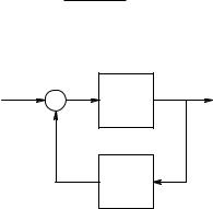
In electronic system design, useful information about the closed-loop behavior of a feedback system may be obtained from the Nyquist test, which is based on the steady-state sinusoidal frequency response of the system’s loop gain function. This test is well suited for design and stability analysis based on experimental frequency response data. As an introduction to the Nyquist test for closed-loop system stability, consider the conventional singleinput, single-output linear feedback system shown in Figure 5.5. In this system, no minus sign assumption is made at the summing point. The closedloop system transfer function is simply:
Y |
(s) = |
G(s) |
G(s) |
|
|
|
[1− AL (s)] |
= |
|
(5.21) |
|
X |
RD(s) |
||||
E
X
FIGURE 5.5
A simple two-block SISO feedback system.
G(s)
H(s)
Y
© 2004 by CRC Press LLC

Feedback, Frequency Response, and Amplifier Stability |
207 |
In a negative feedback system, the loop gain AL(s) = −G(s)H(s), so:
Y |
(s) = |
|
G(s) |
(5.22) |
|
1+ G(s)H(s) |
|||
X |
||||
|
|
[ |
] |
|
The denominator of the closed-loop transfer function is called the return difference, RD(s) ∫ [1 + G(s)H(s)]. If RD(s) is a rational polynomial, as stated earlier, then its zeros are the poles of the closed-loop system function. The Nyquist test effectively examines the zeros of RD(s) to see if any lie in the right-half s-plane. Poles of the closed-loop system in the right-half s-plane produce unstable behavior. In practice, it is more convenient to work with AL(s) = 1 − RD(s) and see if any complex (vector) s values make AL(s) 1–0∞.
The Nyquist test uses a process known as conformal mapping to examine the poles and zeros of AL(s) — thus the zeros of RD(s). In the conformal mapping process used in the Nyquist test, the vector s lies on the contour C1 shown in Figure 5.6. This contour encloses the entire right-half s-plane. The infinitesimal semicircle to the left of the origin is to avoid any poles of AL(s) at the origin. Because the test is a vector test, AL(s) must be written in vector difference form. For example:
A (s) = |
|
K(s + a) |
|
A (s) = |
|
−K(s − s1) |
|
= |
|
K |
|
A |
|
|
|
–θ − θ − θ − π |
||
|
|
|
|
|||||||||||||||
|
(s + b)(s + c) |
|
(s − s2 )(s − s3 ) |
|
B |
|
|
|
C |
|
||||||||
L |
|
L |
|
|
|
|
|
|
a b c |
|||||||||
|
|
|
|
|
|
|
|
|
|
|
|
|
|
|
|
|||
|
|
|
|
|
|
|
|
|
|
|
(5.23) |
|||||||
|
Factored Laplace form |
|
Vector difference form |
|
Vector polar form |
|||||||||||||
The convention used in this text places a (net) minus sign in the numerator of the loop gain when the feedback system uses negative feedback. The vectors s1 = −a, s2 = −b, and s3 = −c are negative real numbers. In practice, s has values lying on the contour shown in Figure 5.6. The vector differences (s − s1) = A, (s − s2) = B, and (s − s3) = C are shown for s = jω1 in Figure 5.7. For each s value on the contour C1, there is a corresponding vector value, AL(s).
A fundamental theorem in conformal mapping says that if the tip of the vector s assumes values on the closed contour, C1, then the tip of the AL(s) vector will also generate a closed contour, the nature of which depends on its poles and zeros.
Before continuing with the treatment of the vector loop gain, it is necessary to go back to the vector return difference, RD(s) = 1 − AL(s), and examine the Nyquist test done on the RD(s) of an obviously unstable system. Assume:
RD(s) = |
K(s − 1) |
RD(s) = |
K(s − s1 ) |
(5.24) |
|
(s − s2 )(s − s3 ) |
|||
(s + 2)(s + 1) |
Recall that a right-half s-plane zero of RD(s) is a right-half (unstable) pole of the closed-loop system. The vector s assumes values on the contour C1′
© 2004 by CRC Press LLC
208 |
Analysis and Application of Analog Electronic Circuits |
j∞
s-plane
C1
R = ∞
jε |
ε |
∞ |
σ |
|
|||
|
|
|
|
−jε |
|
|
|
−j∞
FIGURE 5.6
The contour C1 containing s values traversed clockwise in the s-plane.
in Figure 5.8. Note that C1′ does not need the infinitesimal semicircle around the origin of the s-plane because RD(s) has no poles or zeros at the origin in
this case. Note that as s goes from s = j0+ to s = +j•, the angle of the RD(s) vector goes from +180 to −90∞ and RD(s) goes from K/2 to 0. When s = •,RD(s) = 0 and its angle goes from −90 to +90∞ at s = −j•.
The RD(s) vector contour (locus) in the RD(s) plane is shown in Figure 5.9. Note that the vector locus for s = −jω values is the mirror image of the locus for s = +jω values. It can also be seen in this case that the complete RD(s) locus (for all s values on C1′ traversed in a clockwise direction in the s-plane) makes one net clockwise encirclement of the origin in the RD(s) vector plane. This encirclement is the result of the contour C1′ having enclosed the righthalf s-plane zero of RD(s). The encirclement is the basis for the Nyquist test relation for the return difference:
Z = NCW + P |
(5.25) |
© 2004 by CRC Press LLC

Feedback, Frequency Response, and Amplifier Stability |
209 |
|
|
|
jω |
|
s-plane |
|
|
|
|
|
s = jω1 |
|
A = (s − s1) |
|
|
|
B = (s − s2) |
|
|
|
|
C = (s − s3) |
|
−a |
−b |
−c |
σ |
|
|
|
s3 |
|
|
s2 |
|
|
s1 |
|
|
FIGURE 5.7
The s-plane showing vector differences from the real zero and two real poles of a low-pass filter to s = jω1.
Here Z is the number of right-half s-plane zeros of RD(s) or right-half s-plane poles of the closed-loop system’s transfer function. Obviously, Z is desired to be zero. NCW is the observed total number of clockwise encirclements of the origin by the RD(s) contour. P is the known number of right-half s-plane poles of RD(s) (usually zero).
Now return to the consideration of the more useful loop gain transfer function. Recall that when RD(s) = 0, AL(s) = +1. For the first example, take:
A |
(s) = |
−K(s − 2) |
A |
|
(s) = |
−K(s − s1 ) |
(5.26) |
(s + 5)2 (s + 2) |
|
(s − s2 )2 (s − s3 ) |
|||||
L |
|
|
L |
|
|
Figure 5.10 shows the s-plane with the poles and zeros of AL(s), the contour C1′, and the vector differences used in calculating AL(s) as s traverses C1′ clockwise. Table 5.1 gives values of AL(s) and – AL(s) for s values on C1′.
The polar plot of AL(s) is shown in Figure 5.11. Because AL(s) is used instead of RD(s), the point AL(s) = +1 is critical for encirclements, rather than the origin. The positive real point of intersection occurs for s = j0. It is easily
© 2004 by CRC Press LLC

210 |
Analysis and Application of Analog Electronic Circuits |
|
|
j∞ |
|
|
s-plane |
|
|
|
of RD |
|
|
|
|
C1’ |
|
|
|
s = jω1 |
|
|
s - s2 |
s - s1 |
|
|
s - s3 |
|
|
|
|
∞ |
σ |
−2 |
−1 |
+1 |
|
|
|
R = ∞ |
|
|
|
−j∞ |
|
FIGURE 5.8
The vector s-plane of the return difference showing vector differences and contour C1′ for an RD(s) having a real zero in the right-half s-plane. s traverses the contour clockwise.
seen that if K > 25, one net CW encirclement of the +1 point will take place. The Nyquist conformal equation can be modified to:
PCL = NCW + P |
(5.27) |
PCL is the number of closed-loop system poles in the right-half s-plane. NCW is the total number of clockwise encirclements of +1 in the AL(s) plane as s traverses the contour C1′ clockwise. P is the number of poles of AL(s) known a priori to be in the right-half s-plane. Thus, for the system of the first example, P = 0 and NCW = 1 only if K > 25. The closed loop system is seen to be unstable with one pole in the right-half s-plane when K > 25.
In a second example, the system of example 1 is given positive feedback. Thus:
AL (s) = |
+K(s − 2) |
(5.28) |
(s + 5)2 (s + 2) |
Figure 5.12 shows the polar plot of the positive feedback system’s AL(s) as s traverses the contour C1′. Now if K exceeds a critical value, two clockwise
© 2004 by CRC Press LLC
Feedback, Frequency Response, and Amplifier Stability |
|
211 |
|
|
−270o |
|
|
|
Polar plane |
|
|
|
ω > 0 |
|
|
|
RD |
|
|
|
K/2 ω = 0 |
ωo |
−360o |
−180o |
ω = ∞ |
|
|
|
|
|
|
ω < 0
−450o
FIGURE 5.9
The vector contour in the polar (complex) plane of the RD(s) of Equation 5.24 as s traverses C1′ clockwise.
encirclements of +1 will occur, so two closed-loop system poles will be in the right-half s-plane. Under these conditions, the instability will be a sinusoidal oscillation with an exponentially growing amplitude. To find the critical value of K for instability, it is convenient first to find the s = jωo value at which the system will oscillate by examining the phase of AL(jωo) where AL crosses the positive real axis:
− 2 tan−1(ωo/5) − tan−1(ωo/2) + [180∞ − tan−1(ωo/2)] = 0° |
(5.29A) |
|
|
¬ |
|
− 2 tan−1(ωo/5) − 2 tan−1(ωo/2) = −180∞ |
(5.29B) |
|
|
¬ |
|
tan−1(ω |
/5) + tan−1(ω /2) = 90∞ |
(5.29C) |
o |
o |
|
Trial and error solution of Equation 5.29C yields ωo = 3.162 r/s. Substituting this ωo value into AL(jωo) = +1 and solving for K yields K = 35.00. Therefore, if K > 35, the positive feedback system is unstable, with two net CW encirclements of +1 and thus a complex-conjugate pole pair in the right-half
© 2004 by CRC Press LLC
212 |
|
|
Analysis and Application of Analog Electronic Circuits |
||||
|
|
|
|
jω |
|||
|
|
|
|
j∞ |
|||
|
s-plane |
|
|
|
|
|
|
|
|
|
|
|
|
||
|
of AL(s) |
|
|
|
|
|
|
|
|
|
|
|
C1’ |
||
|
|
|
(s - s2)2 |
|
s = j2 |
||
|
|
|
|
(s − s1) |
|||
|
|
|
|
|
|||
|
|
|
(s − s3) |
|
∞ |
σ |
|
|
|
|
−2 |
|
|
|
|
|
− |
5 |
+2 |
|
|
||
−j∞
FIGURE 5.10
The vector s-plane of the loop gain showing vector differences and contour C1′ for a negative feedback system’s AL(s) having a real zero in the right-half s-plane. s traverses the contour clockwise.
TABLE 5.1
Values of AL(s) as s
Traverses Contour C1′
Clockwise in the s-Plane
s |
ΩAL(s)Ω |
– AL(s) |
±j0 |
+K/25 |
0∞ |
j2 |
K/29 |
−133.6∞ |
j5 |
K/50 |
−226.4∞ |
j• |
0 |
−360∞ |
+• |
0 |
−180o |
−j• |
0 |
+360∞ |
−j2 |
K/29 |
+133.6∞ |
−j5 |
K/50 |
+226.4∞ |
−j• |
0 |
+360∞ |
s-plane. Furthermore, the frequency of oscillation at the threshold of instability is ωo = 3.162 r/s.
As a third and final example of the Nyquist stability criterion, the Nyquist plot of a third-order negative feedback system with loop gain is examined:
© 2004 by CRC Press LLC
Feedback, Frequency Response, and Amplifier Stability |
213 |
−270o |
|
Polar plane |
|
of AL |
|
−j2 |
|
j5 |
|
|
−360o |
−180o |
K/25 ω = +0 |
AL |
|
−j5 |
|
j2 |
|
−90o
FIGURE 5.11
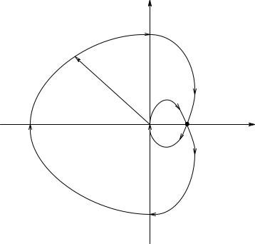
The Nyquist vector contour of the SISO negative feedback system’s AL(s) as s traverses C1′. Note that this type of contour is always symmetrical around the real axis, and is closed because C1′ is also closed. See text for discussion of stability.
AL (s) = |
−Kβ |
(5.30) |
|
s(s + 5)(s + 2) |
|||
|
|
This system has a pole at the origin, so in examining AL(s), s must follow
the contour C1 with the infinitesimal semicircle of radius ε avoiding the origin. Start at s = jε and go to s = j•. At s = jε, AL(s) • and – AL =
–270∞. Because s j•, AL(s) 0 and – AL −450∞. Now when s traverses
the • radius semicircle on C1, AL(s) = 0 and the phase goes through 0∞ and then to +90∞, all with AL(s) = 0. Now as s goes from −j• to −jε, AL(s)
grows larger and its phase goes from +90 to −90∞ (or +270∞). As s traverses the small semicircle part of C1, AL(s) • and the phase goes from −90° to −180∞ at s = ε, and then to −270∞ at s = jε.
The complete contour, AL(s), is shown in Figure 5.13. Note that if Kβ is large enough, there are two CW encirclements of +1 by the AL(s) locus, signifying two closed-loop system poles in the right-hand s-plane and thus oscillatory instability. Because AL(jωo) is real, it is possible to set the imaginary terms in the denominator of AL(jωo) = 0 and solve for ωo. Thus:
jω |
o |
(jω |
o |
+ 5)(jω |
o |
+ 2) = − jω 3 |
− 7ω 2 |
+ 10 jω |
o |
= real |
(5.31) |
|
|
|
o |
o |
|
|
|
and (−jωo3 + 10 jωo) = 0 or ωo = 3.162 r/s and Kβ > 7ωo2 = 70 for instability.
© 2004 by CRC Press LLC
214 |
Analysis and Application of Analog Electronic Circuits |
+90o
Polar plane
 ω = 2
ω = 2
+180o ω = 0+ |
0o |
-K/25 |
+1 |
ω = 5
FIGURE 5.12
The Nyquist vector contour of the SISO positive feedback system’s AL(s) as s traverses C1′. This is the same system as in Figure 5.11, except it has PFB.
5.4Use of Root Locus in Feedback Amplifier Design
Given the knowledge of the positions of the poles and zeros of the loop gain of a linear SISO single-loop feedback system, the root-locus technique allows one to predict precisely where the closed-loop poles of the system will be as a function of system gain. Thus, root locus (RL) can be used to predict the conditions for instability, as well as to design for a desired closed-loop transient response. Many texts on linear control systems treat the generation and interpretation of root-locus plots in detail (Kuo, 1982; Ogata, 1990). Root locus has also been used in the design of electronic feedback amplifiers, including sinusoidal oscillators (Northrop, 1990).
It is often tedious to construct root-locus diagrams by hand on paper, except in certain simple cases described later. Detailed quantitative RL plots can be generated using the Matlab‚ subroutine, “RLOCUS.” Several of the examples in this section are from Matlab plots.
The concept behind the root-locus diagram is simple: Figure 5.14 shows a simple one-loop linear SISO feedback system. The closed-loop gain is:
Y |
(s) = |
C(s)Gp (s) |
= |
C(s)Gp (s) |
(5.32) |
||
X |
|
1+ C(s)G |
(s)H(s) |
||||
|
1− A |
(s) |
|
|
|||
|
|
L |
|
|
p |
|
|
© 2004 by CRC Press LLC

Feedback, Frequency Response, and Amplifier Stability |
215 |
−270o, +90o
∞ @ s = jε
AL
ω = 3.162 r/s
±180o ∞ @ s = ε |
+1 |
−360o, 0o
∞ @ s = −jε
−90o, +270o
FIGURE 5.13
The Nyquist vector contour plot of the NFB AL(s) of Equation 5.30. This AL(s) has a pole at the origin.
X |
E |
U |
Y |
|
|
C(s) |
Gp(s) |
−
H(s)
FIGURE 5.14
A three-block SISO system with negative feedback.
C(s) is the controller transfer function acting on E(s); Gp(s) is the plant transfer function (input U(s), output Y(s)), and H(s) is the feedback path transfer function. The system loop gain is:
AL(s) = −C(s)Gp(s)H(s) |
(5.33) |
(The minus sign indicates that the system uses negative feedback.)
© 2004 by CRC Press LLC

216 |
Analysis and Application of Analog Electronic Circuits |
The RL technique allows one to plot complex s values that make the return difference 0 in the s-plane, thus making the closed-loop transfer function,F(s) •. The s values that make F(s) • are, by definition, the poles of F(s). These poles move in the s-plane as a function of a gain parameter in a predictable, continuous manner as the gain is changed. Because finding s values that set AL(s) = 1–0∞ is the same as setting F(s) = •, the root-locus
plotting rules are based on finding s values that cause the angle of −AL(s) = −180∞ and −AL(s) = 1. The root-locus plotting rules are based on satisfying
the angle or the magnitude condition on −AL(s). The vector format of −AL(s) is used to derive the plotting rules.
For example, first assume a feedback system with the loop gain AL(s) given below. Note the three equivalent ways of writing AL(s):
|
|
|
|
−Kβ |
( |
sτ |
1 |
+ 1 |
|
|
|||||||||
AL |
(s) = |
|
|
|
|
|
|
|
|
|
|
|
|
) |
(time-constant form) |
||||
( |
sτ |
2 |
|
|
|
)( |
sτ |
3 |
) |
||||||||||
|
|
|
|
|
+ 1 |
|
+ 1 |
|
|
||||||||||
AL (s) = |
−Kβτ1 |
|
|
|
|
|
|
|
(s + 1 τ1) |
(Laplace form) |
|||||||||
|
τ2 |
τ3 |
|
|
(s + 1 τ2 )(s + 1 τ3 ) |
||||||||||||||
|
|
|
|
|
|
||||||||||||||
−AL (s) = |
−Kβτ1 |
|
|
|
|
|
(s − s1 ) |
(vector form) |
|||||||||||
|
τ2 |
τ3 |
|
|
(s − s2 )(s − s3 ) |
||||||||||||||
|
|
|
|
|
|
|
|
|
|||||||||||
where s1 = −1/τ1, s2 = −1/τ2, and s3 = −1/τ3. For the magnitude criterion, s must satisfy:
(5.34A)
(5.34B)
(5.34C)
|
|
s − s1 |
|
|
= |
τ |
2 |
τ |
3 |
(5.35A) |
||
|
s − s2 |
|
s − s3 |
|
K βτ1 |
|||||||
|
|
|
||||||||||
|
|
|
|
|
||||||||
and, for the angle criterion, s must satisfy:
θ1 − (θ2 + θ3) = −180∞ |
(5.35B) |
Nine basic root-locus plotting rules are derived from the preceding angle and magnitude conditions and used for pencil-and-paper construction of RL diagrams:
1.Number of branches: there is one branch for each pole of AL(s).
2.Starting points: locus branches start at the poles of AL(s) for Kβ = 0.
3.End points: The branches end at the finite zeros of AL(s) for Kβ •. Some zeros of AL(s) can be at s = •.
4.Behavior of the loci on the real axis (from the angle criterion): For a negative feedback system, on real-axis locus branches exist to the
©2004 by CRC Press LLC
Feedback, Frequency Response, and Amplifier Stability |
|
217 |
||
|
|
|
|
ω |
|
|
|
|
j |
|
|
s-plane |
|
|
|
|
ε |
θ3 |
|
θ1 |
|
θ2 |
σ |
|
|
|
|||
−ω1 |
−ω2 |
−P |
−ω3 |
|
FIGURE 5.15
s-Plane vector diagram illustrating the vectors and angles required in calculating the breakaway point of complex conjugate locus branches when they leave the real axis. (See part 7 of the nine basic root-locus plotting rules in the text.)
left of an odd number of on-axis poles and zeros of AL(s). If the feedback for some reason is positive, then on-axis locus branches are found to the right of a total odd number of poles and zeros of AL(s). (See following examples.)
5.Symmetry: root-locus plots are symmetrical around the real axis in the s-plane.
6.Magnitude of gain at a point on a valid locus branch: from the magnitude criterion, at a vector point s on a valid locus branch:
K β = |
s − s2 |
s − s3 |
τ2 |
τ3 |
(5.36) |
||
|
s − s1 |
τ1 |
|
||||
|
|
|
|
||||
7. Points at which locus branches leave or join the real axis: the breakaway or reentry point is algebraically complicated to find; also, there are methods based on the angle and the magnitude criteria. For example, in a negative feedback system loop gain function with three real poles, two locus branches leave the two poles closest to the origin and travel toward each other along the real axis as K β is raised. At some critical K β, the branches break away from the real axis, one at +90∞ and the other at −90∞. If the angle criterion at the breakaway point, as shown in Figure 5.15, is examined, it is clear that:
−(θ1 + θ2 + θ3) = −180∞ |
(5.37) |
From the geometry on the figure, the angles can be written as arctangents:
tan−1 [ε (ω1 − P)]+ tan−1 [ε
 (ω2 − P)]+ {π − tan−1[ε
 (P − ω3 )]}= π (5.38)
© 2004 by CRC Press LLC

218 Analysis and Application of Analog Electronic Circuits
TABLE 5.2
Asymptote Angles with the Real Axis in the s-Plane
Negative feedback |
|
Positive feedback |
||
N − M |
k |
|
N − M |
k |
1 |
180∞ |
1 |
0∞ |
|
2 |
90∞; 270∞ |
2 |
0∞; 180∞ |
|
3 |
60∞; 180∞; 300∞ |
3 |
0∞; ±120∞ |
|
4 |
45∞; 135∞; 225∞; 315∞ |
4 |
0∞; 90∞; 180∞; 270∞ |
|
|
|
|
|
|
For small arguments, tan−1(x) x, so: |
|
[ε (ω1 − P)]+ [ε (ω2 − P)]− [ε (P − ω3 )]= 0 |
(5.39) |
This equation can be written as a quadratic in P: |
|
3P2 − 2(ω1 + ω2 + ω3 )P + (ω2ω3 + ω1ω2 + ω1ω3 ) = 0 |
(5.40) |
The desired P-root lies between −ω2 and −ω3.
8.Breakaway or reentry angles of branches with the real axis: the loci are separated by angles of 180∞/n, where n is the number of branches intersecting the real axis. In most cases, n = 2, so the branches approach the axis perpendicular to it.
9.Asymptotic behavior of the branches for Kβ •:
(a)The number of asymptotes along which branches approach zeros at s = • is NA = N − M, where N is the number of finite poles and M is the number of finite zeros of AL(s).
(b)The angles of the asymptotes with the real axis are ϕk, where k = 1… N − M. ϕk is given in Table 5.2.
(c) The intersection of the asymptotes with the real axis is a value IA along the real axis. It is given by:
I = (real parts of finite poles)− (real parts of finite zeros) (5.41) |
|
A |
N − M |
|
|
An example of finding the asymptotes and IA is shown in Figure 5.16 This negative feedback system has a loop gain with four poles at s = 0, s = −3,
and a complex-conjugate pair at s = −1 ± j2. There are no finite zeros. Thus, IA = [(−3 − 1 − 1) − (0)]/4 = −5/4. From the table, the angles are ±45∞ and
±135∞. This RL plot was done with Matlab®.
To get a feeling for plotting RL diagrams on paper using the preceding rules, it is necessary to examine several representative examples:
© 2004 by CRC Press LLC
Feedback, Frequency Response, and Amplifier Stability |
|
|
219 |
||||||
5 |
|
|
|
|
|
|
|
|
|
4 |
|
|
|
|
|
|
|
|
|
3 |
|
|
|
|
|
|
|
|
|
2 |
|
|
|
|
|
|
|
|
|
1 |
|
|
|
|
|
|
|
|
|
0 |
|
|
|
|
|
|
|
|
|
–1 |
|
|
|
|
|
|
|
|
|
–2 |
|
|
|
|
|
|
|
|
|
–3 |
|
|
|
|
|
|
|
|
|
–4 |
|
|
|
|
|
|
|
|
|
–5 |
–5 |
–4 |
–3 |
–2 |
–1 |
0 |
1 |
2 |
3 |
–6 |
|||||||||
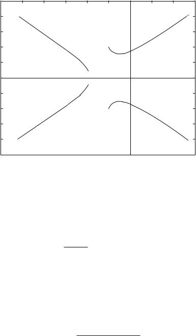
FIGURE 5.16
A Matlab RLocus plot for a negative feedback loop gain with a pole at the origin, a real pole, and a pair of C–C poles.
Example 1 examines the use of root locus in the design of a feedback amplifier using two op amp gain stages, as shown in Figure 5.17(A). This feedback amplifier can never be unstable, but its closed-loop poles can have so little damping that the system is useless. The gain for stage 1 is given by:
Kv1(s) = |
|
V |
= |
|
105 |
|
= |
108 |
|
|
|
2 |
|
−3 |
|
|
|||
|
( |
1 |
1) |
10 |
s + 1 |
|
s + 1000 |
||
|
V |
− V′ |
|
||||||
and the stage 2 gain is given by:
Kv2 (s) = |
V |
= |
−104 |
= |
−2.5 ∞ 106 |
o |
|
|
|||
V |
4 ∞ 10−3 s + 1 |
s + 2.5 ∞ 102 |
|||
|
2 |
|
|
|
|
The NVF system’s loop gain is therefore:
( ) = − β 2.5 ∞ 1014
AL s (s + 103 )(2 + 2.5 ∞ 102 )
(5.42)
(5.43)
(5.44)
The system’s root-locus diagram is shown in Figure 5.17(B). The locus branches begin on the loop gain poles and move parallel to the jω axis in
© 2004 by CRC Press LLC
220 |
Analysis and Application of Analog Electronic Circuits |
|
v1 |
|
v2 |
|
|
|
|
|
|
|
Vo |
+ |
v1’ |
Kv1(s) |
Kv2(s) |
||
|
|
|
|
||
Vs |
|
|
v2’ |
|
|
|
|
|
|
|
|
|
|
|
RF |
|
|
|
R1 β = R1/(R1 + RF) |
|
A |
||
|
|
|
|
|
jω |
|
B |
|
|
|
|
|
|
|
A |
B |
ωn |
|
|
|
|
||
|
|
|
IA |
|
σ |
|
|
|
|
|
|
|
−103 r/s |
−6.25 × 10² |
|
−2.5 × 10² |
|
FIGURE 5.17
(A) Two op amps connected as a noninverting amplifier with overall NVFB. (B) Root-locus diagram for the amplifier. Note that unless a sharply tuned closed-loop frequency response is desired, the feedback gain, β, must be very small to realize a closed-loop system with a damping factor of 0.7071.
the s-plane to ±j• as β increases. The locus branches meet on the negative real axis at s = IA, where they become complex-conjugate:
I = |
(real parts of finite poles)− (real parts of finite zeros) |
|
||
A |
|
|
N − M |
|
|
|
|
|
|
|
|
−103 − 2.5 ∞ 102 |
(5.45) |
|
|
= |
= −6.25 ∞ 102 |
||
|
|
|||
|
2 |
|
|
|
© 2004 by CRC Press LLC

Feedback, Frequency Response, and Amplifier Stability |
221 |
It is desirable for the closed-loop system to have poles at P and P* so that its damping factor will be ξ = 0.7071. From the geometry of the RL plot, the closed-loop ωn = 6.25 ∞ 102 ∞ 2 = 8.84 ∞ 102 r/s. From the RL magnitude criterion, find the β value to place the closed-loop poles at P and P*:
|
−AL |
(s = P) |
|
= 1 = |
βp 2.5 ∞ 1014 |
(5.46) |
|||
|
|
||||||||
|
|
|
|||||||
|
|
|
|
A |
B |
|
|
||
|
|
|
|
|
|
|
|
||
The vectors A and B are defined in the figure and Pythagoras indicates:
|
A |
|
= |
|
B |
|
= (6.25 ∞ 102 )2 + (3.75 ∞ 102 )2 = 7.289 ∞ 102 |
(5.47) |
|
|
|
|
Thus, the value
β |
|
= |
(7.289 ∞ 102 )2 |
= 2.125 ∞ 10−9 |
(5.48) |
|
p |
2.5 ∞ 1014 |
|||||
|
|
|
|
will give the closed-loop system a damping factor of 0.707. The feedback amplifier’s closed-loop dc gain is:
A |
|
(0) = + |
109 |
|
= 3.20 ∞ 108 |
(5.49) |
|
v |
1+ 2.125 ∞ 10−9 |
∞ 109 |
|||||
|
|
|
|
In summary, the cascading of two compensated op amps given a single feedback loop gives a closed-loop amplifier with high gain but relatively poor bandwidth. As an exercise, consider the −3-dB bandwidth possible if two noninverting op amp amplifiers, each with its own NVF, are cascaded such that their combined dc gain is 3.20 ∞ 108.
Example 2 examines the commonly encountered circle root locus. The negative feedback system’s loop gain transfer function has two real poles and a real zero:
AL |
(s) = |
−Kp |
β(s + a) |
(5.50) |
|
(s + b)(s + c) |
|||||
|
|
|
|||
where a > b > c > 0.
Angelo (1969) gave an elegant proof that this system’s root locus does indeed contain a circle centered on the zero of AL(s). The circle’s radius R is shown to be the geometrical mean distance from the zero to the poles, i.e.,
R = (a − b)(a − c) |
(5.51) |
The breakaway and reentry points are easily found from a knowledge that the circle has a radius R and is centered at s = −a. The circle root locus is shown in Figure 5.18(A).
© 2004 by CRC Press LLC
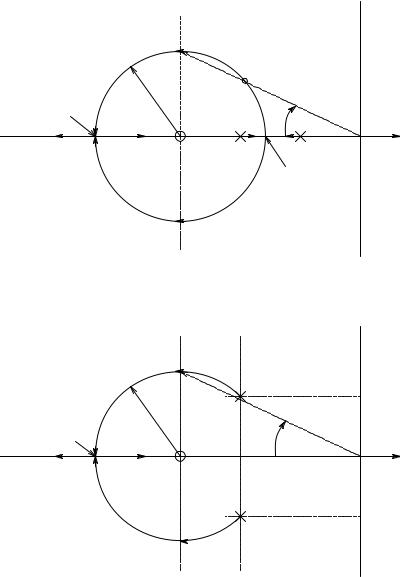
222 |
Analysis and Application of Analog Electronic Circuits |
 jω
jω
s-plane
|
P |
|
P’ |
R |
ωn |
−(a + R)
φ |
σ |
|
−a |
−b |
−c |
−(a − R)
A
 jω
jω
|
|
|
s-plane |
|
|
|
P |
|
|
|
|
|
|
+jγ |
|
R |
|
ωn |
|
|
|
|
|
|
−(a + R) |
|
|
φ |
σ |
|
|
|
||
|
|
−a |
−α |
|
|
|
|
|
|
|
|
|
|
−jγ |
B
FIGURE 5.18
(A) The well-known circle root locus for a NFB system with two real poles an a high-frequency real zero. See text for discussion. (B) Interrupted circle root locus for the same NFB system with complex-conjugate poles at s = −α ± jγ.
If the loop gain’s poles are complex-conjugate, the root locus is an interrupted circle, shown in Figure 5.18(B). The circle is still centered on the zero at s = −a. The poles are at s = −α ± jγ. The AL(s) is:
© 2004 by CRC Press LLC