TABLE 2.2

Semiconductor LED Materials and Approximate Emission

Peak Wavelengthsa

a Peak emission, λ, depends on temperature and diode current.

561 nm and the half-intensity width is measured at approximately 26 nm, giving an LED Q = 21.6.

Modern LEDs are now available in the near UV, which provides excellent application in biochemical fluorescence analysis as an inexpensive source of excitation for DNA microarrays (gene chips) and many other modes of fluorescent chemical analysis. Their UV can also be used to catalyze the polymerization of dental fillings and for spot sterilization. For example, the Nichia NSHU550E UV LED (gallium indium nitride) has a spectral emission peak centered at 370 nm, quite invisible to the human eye. Nichia also makes gallium nitride (GaN) single quantum well LEDs that emit blue with a peak at approximately 470 nm that are intended for excitation in fluorescence applications, including protein analysis and DNA analysis using SYBR“ green and SYPRO“ orange molecular tags.

The following section shows that laser diodes (LADs) have much narrower spectral emission lines, but also can have under certain operating conditions many closely spaced emission lines.

2.6.7Laser Diodes

The basic difference between an LED and an LAD is that the latter has an optical resonance cavity that promotes lasing. The optical cavity has two end facet partial mirrors that reflect photons back into the cavity so that a selfsustaining laser action occurs. The mirrors can be the cleaved surfaces of the semiconductor crystals or may be optically ground, polished, and coated. The LAD unit generally contains a photodiode (PD) that is used with an external circuit to monitor the optical power output, Po , of the LAD. LADs are easily damaged by excess ID causing excess Po . Often the PD output is used to provide feedback to limit the optical power output of the LAD so that the end mirrors are not damaged by heat or XS light. If the end mirrors are damaged, the LAD becomes an expensive, ineffective LED.

© 2004 by CRC Press LLC

FIGURE 2.69

(A) iD vs. vD curve for a GaP (green) LED. Note the high threshold voltage for forward conduction. (B) For comparison, the iD vs. vD curve for a typical Si small-signal pn diode. (C) Relative light intensity vs. forward current.

Low-power LADs come in a variety of packages; probably the most familiar is the cylindrical can with top (end) window. Such TO-cans are typically 5.6 or 9.0 mm in diameter and have three leads: (1) common, (2) LAD cathode, and (3) PD anode. The PD’s cathode and the LAD’s anode are connected to the common lead.

© 2004 by CRC Press LLC

FIGURE 2.70

Spectral emission characteristic of a GaP green LED.

How does diode lasing occur? If some forward current, ID, generates an electron–hole pair ready to emit a photon of energy Eg = hνo and another photon is present with energy hνo, the existing photon stimulates the elec- tron–hole pair to recombine and to emit a photon coherent to the existing one. The probability of stimulated emission is proportional to the density of excess electrons and holes in the active region and to the density of photons. Under low-density conditions, it is negligible. However, if coherent positive feedback is provided by reflecting back some exiting photons with the end mirrors, the stimulated emission can become self-sustaining. This self-sus- taining, stimulated emission is the heart of the laser principle.

Several LAD structures are currently used. Early LAD design used homojunction architecture, the boundary between the p- and n-materials serving as the active (laser) region. The length of the active region was much longer (300 to 1000 μm) than its thickness (1 μm) or width (3 μm). The end facets served as the mirrors. A LAD design using alternating layers of p- and n-materials is called a heterojunction structure. For example, if three p-layers are alternated with three n-layers, there are five active regions to lase. When four p-layers are alternated with four n-layers, there are seven active regions, etc. Heterojunction designs have been used to fabricate high-power output LADs. Because of their geometry (long and very thin) homoand heterojunction LAD output beams tend to be asymmetrical and are often difficult to focus into a small symmetrical (Gaussian) spot.

© 2004 by CRC Press LLC

The new, vertical cavity, surface-emitting laser (VCSEL) diodes consist of a (top) light exit window (it can be round, 5 to 25 μm in diameter), a topdistributed Bragg reflector, a gap to set the emission wave length, two λ-spacers surrounding a GaAs active region, and then a bottom-distributed Bragg reflector sitting on the bottom substrate. VCSEL lasers operate in a single longitudinal mode. They can be designed to have anastigmatic Gaussian beams, which are easy to focus with simple lenses. Because the mirror area is larger, VCSEL lasers are not as prone to overpower damage and optical feedback is not necessary as it is in edge-emitting LADs. They also lase at much lower IDs because of their efficient mirrors.

LADs are considered to be current-operated devices; they should be driven from regulated current sources, not voltage sources. Figure 2.71(A) illustrates the optical output power, Po, from a LAD vs. the forward current, ID, for a typical heterojunction LAD. IDt is the threshold current where enough elec- tron–hole pairs are produced to sustain lasing. Note that increasing device temperature moves the Po(ID) curve to the right. The steep part of the curve is essentially linear and is characterized by its slope: Po/ ID = ρ watts/amp. In the region of ID between 0 and IDt, the LAD is basically a LED. An algebraic model for the Po(ID) curve above IDt is:

where Px is the intersection of the approximate line with the negative Po axis. Needless to say, IDt is much lower for a VCSEL LAD. (An Avalon, AVAP760, VCSEL, 760-nm LAD has IDt = 2.0 mA and IDQ = 3.0 mA. IDQ is the operating current for this LAD.)

Although VCSEL LADs have a single mode output (the preceding 760-nm VCSEL has a line Q of 3.95 ∞ 1014 Hz/100 ∞ 106 Hz = 3.95 ∞ 106), homoand heterojunction LADs generally emit a multimode “comb” spectral output. The number of spectral lines that appear at the output of a gain-guided LAD depends on the properties of the cavity and mirrors, the operating current, and the temperature. According to the Newport Photonics Tutorial (2003):

The result is that multimode laser diodes exhibit spectral outputs having many peaks around their central wavelength. The optical wave propagating through the laser cavity forms a standing wave between the two mirror facets of the laser. The period of oscillation of this curve is determined by the distance L between the two mirrors. This standing optical wave resonates only when the cavity length L is an integer number m of half wavelengths existing between the two mirrors. In other words, there must exist a node at each end of the cavity. The only way this can take place is for L to be exactly a whole number multiple of half wavelengths λ/2. This means that L = m(λ/2), where λ is the wavelength of light in the semiconductor matter and is related to the wavelength of light in free space through the index of refraction n by the relationship λ = λo/n. As a result of this situation there can exist many longitudinal modes in the cavity of the laser diode, each resonating at its distinct

© 2004 by CRC Press LLC

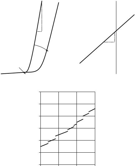
FIGURE 2.71

(A) Optical power output from a laser diode (LAD) vs. forward current. Note that increasing the heterojunction temperature decreases the output power at constant ID. (B) Increase in output wavelength of an LAD at constant Po with increasing case temperature. (C) Mode-hopping behavior of LAD output wavelength with increasing case temperature.

wavelength of λm = 2L/m. From this [development] you can note that two adjacent longitudinal laser modes are separated by a wavelength [difference] of Δλ = λo2/(2nL).

© 2004 by CRC Press LLC

Even single-mode devices [VCSEL LADs] can support multiple [output] modes at low output power… As the operating current is increased, one mode begins to dominate until, beyond a certain operating power level, a single narrow linewidth [output] spectrum appears.

It is also noted that the center λ of an LAD’s output increases with operating temperature. This property is useful in spectroscopy in which the fine struc-

ture of a molecular absorbance spectrum is being studied. Newport gives data for one LAD with a center frequency of 837.6 nm at 20∞C. The center

wavelength increases linearly with increasing temperature to 845.5 nm at 50∞C. Thus, Δλ/ T = 0.263 nm/∞C.

Single-mode LADs can exhibit a phenomenon known as mode-hopping. Here the output λ increases linearly over a short temperature interval, at the upper end of which it hops discontinuously to a slightly larger λ. The linear behavior again occurs, followed by another hop, etc. The linear behavior of λ(T) and mode-hopping are shown in Figure 2.71(B) and Figure 2.71(C). Because of mode-hopping and λ drift with temperature, LADs used for wave length critical applications are temperature stabilized to approximately 0.1∞C around a desired operating temperature using thermoelectric (Peltier) cooling.

Many circuits have been developed to drive LADs under constant-current conditions. Some circuits use the signal from the built-in PD to stabilize the diode’s Po when CW or pulsed output is desired. In communications applications, in which the LAD is driving an optical fiber cable, it is desirable to on/off modulate Po at very high rates, up into the gigahertz in some cases. In biomedical applications, in which the LAD is used as a source for spectrophotometry, the intensity modulation or chopping of the beam is more conveniently done at audio frequencies to permit the operation of lock-in amplifiers, etc.

One of the more prosaic applications of LADs is the common (CW) laser pointer. Some of these devices are operated without any regulation by the simple expedient of using one current-limiting resistor in series with the two

batteries. The resistor is chosen so that ID is always less than IDmax when the batteries are fresh. Of course the pointer spot gets dimmer as the batteries

become exhausted. Figure 2.72 illustrates this basic series circuit and the solution of the LAD’s ID = f (VD) curve with the circuit’s load line.

An example of a two-BJT regulator used in laser pointers (Goldwasser, 2001) is shown in Figure 2.73. This is a type 0, negative feedback circuit that makes Po relatively independent of VB and T. Inspection of this circuit shows that if Po increases, the PD’s IP increases, decreasing IB2, thus IB1 and ID, and thus reducing Po; therefore, negative feedback stabilizes Po.

When it is desired to modulate an LAD at hundreds of megahertz to gigahertz for communications applications, very special circuits indeed are used. LADs can be modulated around some 50% Po point much faster than from fully off to fully on. Several semiconductor circuit manufacturers offer high-frequency single-chip LAD regulator/drivers. For example, the Analog

© 2004 by CRC Press LLC

ID

Max ID

IDQ

FIGURE 2.72

Top: LAD powered from a simple DC Thevenin circuit. Bottom: an LAD’s iD vs. vD curve showing max iD, load lines, and operating point.

FIGURE 2.73

A simple LAD Po (thus iD) regulator circuit. The LAD’s built-in PD is used to make a type 0 intensity controller.

© 2004 by CRC Press LLC

V2

Po

RD

(VCCS)

hν

R

LAD PD

R VL

−VL

FIGURE 2.74

A type 1 feedback system designed by the author to regulate and modulate LAD Po. The LAD’s built-in PD is used for feedback.

Devices AD9661A driver chip allows LAD on/off switching up to 100 MHz, and has <2 ns rise/fall times. The Maxim MAX3263 is a 155 Mbps LAD driver with <1 ns rise/fall times. Needless to say, getting an LAD to switch at such rates involves the artful use of ferrite beads, as well as consideration of parasitic distributed parameters such as LAD lead inductance and stray capacitances. The MAX3263 chip also has a “slow start” feature to protect the LAD at turn-on. The design of GHz modulation circuits is beyond the scope of this text and will not be treated here.

Figure 2.74 illustrates the architecture of an op amp feedback/modulation circuit designed by the author for spectrophotometric LAD applications. It uses a VCCS to drive the LAD and a feedback loop containing signal conditioning for the on-board PD, a difference amplifier (DA), an integrator, and another DA. The input that sets the LAD’s output power is VoQ, which can be an audio-frequency square-wave, a sinewave + DC, or just DC. The VCCS subunit drives the LAD. Its transconductance can be found by KVL, noting:

The node equation for the power op amp’s summing junction can be written:

© 2004 by CRC Press LLC

Now refer to the block diagram shown in Figure 2.75, which illustrates the simplified dynamics of the circuit of Figure 2.74. The LAD’s Po(ID) curve for ID > IDt is approximated by the linear relation of Equation 2.211. The output of the PD conditioning amplifier is subtracted from the set-point, VoQ, to create an error voltage, Ve, which is integrated forming V3. V3 is then subtracted from V1 > 0, a bias voltage, forming Vc, the input to the VCCS. ID is the LAD drive current. Application of Mason’s rule yields the transfer function:

Note that V1 and Px are dc levels. At turn-on, they can be considered to be steps. Using the Laplace initial value theorem:

© 2004 by CRC Press LLC