The SNRo clearly has a maximum with respect to the turns ratio, n. (It can be shown that F is minimum when n = no, so SNRo is maximum (Northrop, 1997). If the denominator of Equation 9.60 is differentiated with respect to n2 and set equal to zero, an optimum turns ratio, no, exists that will maximize SNRo. no is given by:

If the noiseless (ideal) transformer is given the turns ratio of no, then it is easy to show that the maximum output SNR is given by:

The general effect of transformer SNR maximization on the system’s noise figure contours is to shift the locus of minimum NFspot to a lower range of Rs; no obvious shift occurs along the fc axis. Also, the minimum NFspot is higher with a real transformer because a practical transformer is noisy, as discussed earlier. As a rule of thumb, using a transformer to improve output

SNR and reduce NFspot is justified if (ena2 + ina2 Rs2) > 20 ena ina Rs in the range of frequencies of interest (Northrop, 1990).

9.5Cascaded Noisy Amplifiers

9.5.1Introduction

To achieve the required high gain required for certain biomedical signal conditioning applications, it is often necessary to place several IC gain stages in series. A natural question to ask is whether all the component IC gain stages need to be low noise in the low-noise amplifier design. The good news is that as long as the headstage (input, or first stage) is low noise and has a gain magnitude of ≥10, the remaining gain stages do not need to be low noise in design. The headstage’s noise sets the noise performance of the complete signal conditioning amplifier.

© 2004 by CRC Press LLC

+

vs

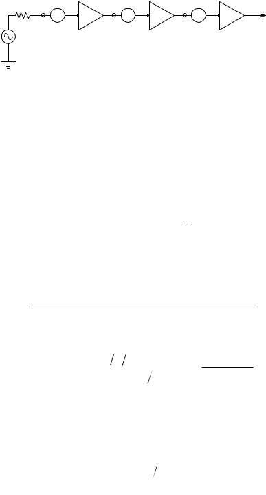
FIGURE 9.13

Three cascaded noisy amplifiers.

9.5.2The SNR of Cascaded Noisy Amplifiers

Figure 9.13 illustrates three cascaded amplifier stages. The amplifier’s overall

gain is KV = KV1 KV2 KV3. The first stage has a white, short-circuit voltage, root power spectrum of ena1 RMSV/ Hz and an input current noise root power spectrum of ina1 RMS V/ Hz. The other two stages have voltage noises

of ena2 and ena3, respectively, and zero current noises. (It can be assumed that the current noises are zero because the output resistance of the previous

stages is assumed to be very low, so that ina2 Ro1 ena2, and ina3 Ro2 ena3.) Assume a sinusoidal input signal, vs(t) = Vs sin(2πft); thus, the MS input

voltage is Vs2/2. The MS output voltage is simply vos2 = (Vs2/2)(KV1KV2KV3)2. The total MS noise output voltage is the sum of the MS noise components

Thus, the SNRo of the three-stage cascaded amplifier is set by the headstage alone, as long as the headstage gain KV1 > 10.

What if the headstage is of necessity a source or emitter follower with near-unity gain? If the preceding equation is examined, it can be seen that it reduces to a lower value for KV1 1, e.g.,

© 2004 by CRC Press LLC

FIGURE 9.14

Equivalent input circuit for a noisy differential amplifier. In this model, both input transistors make noise.

Now the second stage’s voltage noise, ena2, becomes important and KV2 that should be >10; the first and the second stages must use low-noise amplifiers.

9.6Noise in Differential Amplifiers

9.6.1Introduction

As Chapter 3 discussed, the headstage of a differential amplifier contains two active elements (BJTs, JFETs, or MOSFETs) and thus two, independent, uncorrelated sources of ena and ina. The equivalent input circuit of a DA is shown in Figure 9.14. To simplify analysis, the two amplifier input resistances that appear in parallel with the inas have been set to infinity (i.e.,

where AD is the scalar difference-mode gain; AC is the scalar common-mode gain; vid is the difference-mode input signal; and vic is the common-mode input signal. By definition:

© 2004 by CRC Press LLC

Also recall that the common-mode rejection ratio for the simple DA could be expressed as:

Under normal operating conditions, AD AC and CMRR 1.

9.6.2Calculation of the SNRO of the DA

Referring to Figure 9.14, the DA noise model circuit has six independent, uncorrelated noise sources. Thus the total noise PDS at the vi node can be written:

Similarly, the total noise PDS at the vi′ node is:

To find the MS SNRo of the noisy DA, assume that the input signal is pure

DM. Thus vic = 0, vid = vs, and vos2 = AD2 vs2 MSV. To find the MS noise output, set vs = vs′ = 0 and consider that the six noise sources add in quadrature (in

an MS sense). First, note that in the time domain:

and

When the expressions for vi(t) and vi′(t) from Equation 9.70 and Equation 9.71 are substituted into Equation 9.72 and the expectation or mean is taken, cross terms between vi and vi′ vanish because of statistical independence and no correlation. Also, the means of self-cross terms such as ena′(ina′Rs′) also

vanish for the same reasons. Recall that because the DA is symmetrical, ena = ena′ RMSV/ Hz, ina = ina′ RMSA/ Hz and Rs = Rs′. After some algebra that

will not be reproduced here, the MS output noise is given by:

© 2004 by CRC Press LLC