A

R

(E)

+

−

(R)

B

FIGURE 1.7

(A) Equivalent circuit of an intracellular glass microelectrode in a cell, including the equivalent circuits of the AgΩAgCl electrodes. Note the dc half-cell potentials of the electrodes and at the microelectrode’s tip. The tip of the microelectrode is modeled by a lumped-parameter, nonuniform, R–C transmission line. (B) For practical purposes, the ac equivalent circuit of the glass micropipette electrode is generally reduced to a simple R–C low-pass filter.

Typical values of circuit parameters are Rμ 2 ∞ 108 Ω, Cμ 1 ∞ 10−12 F. Thus fb 796 Hz. This is too low a break frequency to reproduce a nerve action potential faithfully, which requires at least a dc to 3-kHz bandwidth. To obtain the desired bandwidth, capacitance neutralization is used (capacitance neutralization is described in Section 4.5.2 of Chapter 4). As shown in Section 9.8.4 in Chapter 9, capacitance neutralization adds excess noise to the amplifier output.

1.9Exogenous Bioelectric Signals

The preceding sections have shown that endogenous bioelectric signals are invariably small, ranging from single microvolts to over 100 mV. Their bandwidths range from dc to perhaps 10 kHz at the most. Signals such as ECG

© 2004 by CRC Press LLC

and EEG require approximately 0.1 to 100 Hz. Exogenous signals on the other hand, can involve modalities such as ultrasound, which can use frequencies from hundreds of kilohertz to tens of megahertz, depending on the application. Ultrasound can be continuous wave (CW) sinusoidal, sinusoidal pulses, or wavelets. The purpose here is not to discuss the details of how ultrasound is generated, received, or processed, but rather to comment on the frequencies and signal levels of the received ultrasound.

Reflected ultrasound is picked up by a piezoelectric transducer or transducer array that converts the mechanical sound pressure waves at the skin surface to electrical currents or voltages. Concern for damaging tissues with the transmitted ultrasound intensity (cells destroyed by heating or cavitation) means that input sound intensity must be kept low enough to be safe for living tissues, organs, fetuses, etc., yet high enough to give a good output signal SNR from the reflected sound energy impinging on the receiving transducer. Many ultrasound transducers are used at ultrasound frequencies below their mechanical resonance.

In this region of operation, the transducer has an equivalent circuit described by Figure 1.8. Cx is the capacitance of the transducer, which of course depends on thickness, dielectric constant of its material, and area of the metal film electrodes; Cx is generally on the order of hundreds of picofarads. Gx is the leakage conductance of the piezomaterial and also depends on the material and its dimensions. Expect Gx on the order of 10−13 S. The coaxial cable connecting the transducer to the charge amplifier has some shunt capacitance, Cc, which depends on cable length and insulating material; it will be on the order of approximately 30 pF/m. Similarly, the cable has some leakage conductance, Gc, which again is length and material dependent; Gc will be about 10−11 S. Finally, the input conductance and capacitance of the electrometer op amp are about Gi = 10−14 S and Ci = 3 pF.

The circuit of Figure 1.8 is a charge amplifier, which effectively replaces

(Cx + Cc + Ci) and (Gx + Gc + Gi) with CF and GF in parallel with the transducer’s Norton current source. Thus the low-frequency behavior of the sys-

tem is not set by the poorly defined (Cx + Cc + Ci) and (Gx + Gc + Gi) but rather by the designer-specified components GF and CF. (Analysis of the circuit is carried out in detail in Section 6.6.3 of Chapter 6.) Note that the Norton current source, ix, is proportional to the rate of change of the ultrasound pressure waves impingent on the bottom of the transducer. The constant d has the dimensions of coulombs/newton. The charge displaced inside

the transducer is given by q = d F. The Norton current is simply ix ∫ q· = d F· =

·

d PA. If the op amp is assumed to be ideal, then the summing junction is at 0 V and, by Ohm’s law, the op amp’s output voltage is

© 2004 by CRC Press LLC

Voc

(Metal film electrodes)

Piezo-transducer

Ultrasound gel

Skin

Tissue

Pi

(Cable)

FIGURE 1.8

Top: Cross-sectional schematic of a piezoelectric transducer on the skin surface. The gel is used for acoustic impedance matching to improve acoustic signal capture efficiency. Pi is the sound pressure of the signal being sensed. Bottom: Equivalent circuit of the piezosensor and a charge amplifier. See text for analysis.

The area A is in m2. The parameter d varies considerably between piezomaterials and also depends on the direction of cut in natural crystals such as quartz, Rochelle salt, and ammonium dihydrogen phosphate. For example, d for X-cut quartz crystals is 2.25 ∞ 10−12 Cb/N and d for barium titanate is approximately 160 ∞ 10−12 Cb/N.

Now consider the mid-frequency output of the charge amplifier when using a lead–zirconate–titanate (LZT) transducer having d = 140 ∞ 10−12 Cb/N, given a sound pressure of 1 dyne/cm2 = 0.1 Pa; A = 1 cm2 = 10−4 m2; and CF = 100 pF.

© 2004 by CRC Press LLC

Thus, received voltage levels in piezoelectric ultrasonic systems are very low. Considerable low-noise amplification is required and band-pass filtering is necessary to improve signal-to-noise ratio. Not included in the preceding analysis is the high-frequency response of the charge amplifier, which is certainly important when conditioning low-level ultrasonic signals in the range of megahertz. (See Section 6.6.3 in Chapter 6 for high-frequency analysis of the charge amplifier.)

1.10 Chapter Summary

This chapter has stressed that endogenous biomedical signals, whether electrical such as the ECG or EEG, or physical quantities such as blood pressure or temperature, vary relatively slowly; their signal bandwidths are generally from dc to several hundred Hertz and, in the case of nerve spikes or EMGs, may require up to 2 to 4 kHz at the high end. All bioelectric signals are noisy — that is, they are recorded in the company of broadband noise arising from nearby physiological sources; in many cases (e.g., EEG, ERG, EOG, and ECoG), they are in the microvolt range and must compete with amplifier noise. In the case of a skin-surface EMG, the recorded signals are the spa- tio–temporal summation of many thousand individual sources underlying the electrodes, i.e., many muscle fibers asynchronously generating action potentials as they contract to do mechanical work. In the case of the scalprecorded EEG, many millions of cortical neurons signal by spiking or by slow depolarization as the brain works, generating a spatio–temporally summed potential between pairs of scalp electrodes.

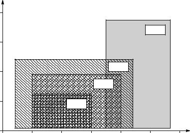
On the other hand, the electrical activity from the heart is spatially localized. The synchronous spread of depolarization of cardiac muscle during the cardiac cycle generates a relatively strong signal on the skin surface, in spite of the large volume conductor volume through which the ECG electric field must spread. Figure 1.9 illustrates the approximate extreme ranges of peak signal amplitudes and the approximate range of frequencies required to condition EOG, EEG, ECG, and EMG signals. Note that the waveforms that contain spikes or sharp peak transients (ECG and EMG) require a higher bandwidth to characterize.

Exogenous biomedical instrumentation signals, such as diagnostic and Doppler ultrasound and signals from MRI systems, were shown to require bandwidths into the tens of megahertz and higher. Amplifiers required for

conditioning such exogenous signals must have high gain bandwidth products (fT), and high slew rates (η), as well as low noise.

© 2004 by CRC Press LLC

FIGURE 1.9

Approximate RMS spectra of four classes of bioelectric signals. Peak expected RMS signal is plotted vs. extreme range of frequencies characterizing the signal.

© 2004 by CRC Press LLC