Examine the system design with practical numbers: let φm ∫ 10º; Ki = 1 and KP = 8.0E−6 sec/V; and 720/c = 2.40E−6. These numbers give a reasonable range sensitivity:

From Equation 12.47, the velocity sensitivity is also useful:

The VPC steady-state output frequency at a 1-m range is 4.17 MHz; when L = 100 m, it is 41.7 kHz.

12.4.6Summary

There are a variety of architectures for voltage-controlled oscillators, including “linear” VCOs using variable gain elements, switched integrating capacitor VCOs, and emitter-coupled, astable multivibrators. Versions of the latter architecture have been made to oscillate in the gigahertz. Another VHF–UHF VCO architecture (not shown here) makes use of the varactor diode (VD). The VD is a reverse-biased pn junction diode in which the diode depletion capacitance is controlled by the reverse-bias voltage. This voltage-variable capacitance can be used to tune oscillators such as the familiar Hartley design and to generate NBFM by adding the modulating signal to the reverse diode bias voltage. VCOs are used in all phase-lock loops and in FM communications applications, as well as in many instrumentation systems.

The voltage-to-period converter (VPC) is a VCO in which the output oscillation’s period is linearly proportional to the input voltage. The VPC is a useful circuit component in a closed-loop, constant-phase laser velocimeter and ranging system. The same closed-loop, constant-phase architecture can also be used with sound or ultrasound to measure object range and velocity simultaneously.

12.5 Phase-Locked Loops

12.5.1Introduction

A phase-locked loop (PLL) (also called a phase-lock loop) is a closed-loop feedback system in which the phase of the PLL’s periodic output is made to follow the phase of a periodic input signal. The closed-loop PLL system’s

© 2004 by CRC Press LLC

Vφ (θ1 − θo)

A

Linearized PD

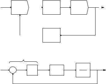
FIGURE 12.24

(A) Basic architecture of a phase-locked loop (PLL). (B) Systems block diagram of a PLL.

natural frequencies are, in general, several orders of magnitude lower than the frequency of the input signal. Phase-lock loops have many applications in communications, control systems, and instrumentation systems. They can be used to modulate and demodulate narrow-band FM (NBFM) signals; demodulate double-sideband/suppressed carrier (DSBSC) signals; demodulate AM signals; generate a frequency-independent phase shift; measure frequencies, including heart rate; synthesize signals used in digital communications systems; detect touch-tone frequencies and status signals used in telephony; control motor speed, etc.

The basic architecture of a PLL is shown in Figure 12.24(A). It includes a phase (difference) detector (PD), loop filter, VCO (VFC), and, sometimes, a frequency divider between the VCO and the PD. (Phase detectors were described in Section 12.3.) A phase detector returns an average voltage proportional to the phase difference between the input signal and the VCO output.

Analysis of PLL dynamics is done assuming lock, i.e., that the input and VCO frequencies are equal. When a PLL first acquires its input signal, f1 π fo and the loop must attain lock through a nonlinear process known as acquisition. The time required for acquisition is important in such PLL applications as telephone touch-tone decoding and the demodulation of FSK signals. Empirical formulas for acquisition times can be found in Northrop (1990) and Gardner (1979).

© 2004 by CRC Press LLC

12.5.2PLL Components

As mentioned earlier, phase detectors such as those used in PLLs have already been considered in Section 12.3. Most IC PLLs use PDs in which the analog input signal is effectively multiplied by a ±1 square wave derived from the VCO. This type of PD is a quadrature detector; the zero phase error condition requires that θ1 − θo = π/2. Analog multiplier and exclusive OR PDs are also quadrature detectors. Only the RSFF PD and the MC 4044 PD are in-phase detectors.

All PDs produce an analog output whose average value, Vφ, is proportional to sin(θe) or to θe. When θe < 15º, sin(θe) can be replaced with θe in radians. Thus, for small-signal errors at lock, the PLL can be modeled by the block diagram in Figure 12.24(B). The VCO is modeled in the frequency domain by Kv s because ωo = Vc Kv r/s and its output phase is, in general, the integral of its output frequency, i.e., θo = ωo dt. The PLL’s dynamics in response to changes in θ1 are determined in part by its closed-loop poles, which can be found from its linear loop gain using root-locus techniques. The PLL’s loop gain is generally:

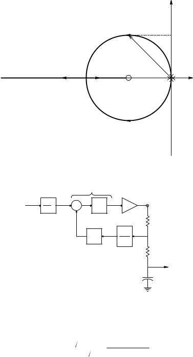
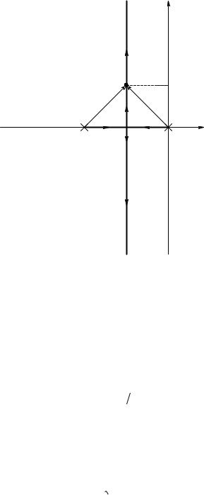
If F(s) = Kf (s + a)/s, then the loop gain function has a zero at s = −a, and two poles at the origin. Its root-locus is the well-known circle, shown in Figure 12.25. Effective design of this PLL wants the closed-loop poles at s = −a ± ja. This gives a damping factor of ξ = 0.707 and an undamped natural frequency of ωn = a2. The scalar gain product, Kp Kf Kv, is adjusted to obtain these closed-loop parameters. It can be shown that Kp Kf Kv = 2a will put the closed-loop poles at s = −a ± ja (Northrop, 1990).

The PLL’s loop filter is generally low-pass and can be of the form F(s) = Kf (s/b + 1), Kf (s + a)/s, Kf (s/a + 1)/(s/b + 1), etc. The loop filter is generally chosen to give the PLL the desired dynamic response in tracking changes in θ1. The PLL’s VCO can have a digital (TTL) or sinusoidal output. The VCO used on IC PLLs often uses the voltage-controlled, emitter-coupled astable multivibrator architecture (see above).

12.5.3PLL Applications in Biomedicine

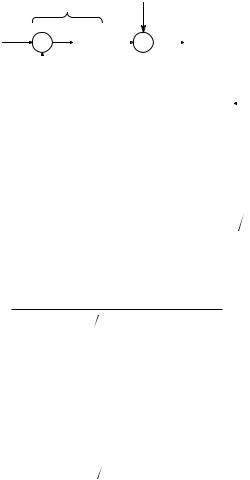
One application of a PLL is its use to measure heart rate. Figure 12.26 illustrates the block diagram of a 4046 CMOS PLL used as a cardiotachometer (Northrop, 1990). The loop filter’s transfer function is found from the voltagedivider relation:

© 2004 by CRC Press LLC

jω

s-plane

ja

ωn = a√2

−a

FIGURE 12.25

Root-locus diagram of a PLL having a loop filter of the form, F(s) = Kf (s + a)/s.

Vo

C

FIGURE 12.26

Block diagram of a PLL used as a heart rate monitor. Vo is proportional to the average heart rate.

Similarly, the output transfer function is:

and the PLL’s loop gain is:

© 2004 by CRC Press LLC

FIGURE 12.27

Block diagram of a PLL used to generate a frequency-independent phase shift. (θi − θo) Vp.

The PLL’s transfer function is thus:

The denominator of the preceding equation is of the standard quadratic form: s2 ωn2 + s 2ξ ωn + 1. Thus:

Examine system ωn, ξ, and dc gain given the typical circuit parameters: Kp = 8.33; Kv = 3.14; N = 4; C = 1.E−5; R1 = 62k; and R2 = 150k. These values yield: ωn = 1.76 r/s; ξ = 1.45 (overdamped); and dc gain Vo/f1 = 8.00 volts/beat/sec = 0.133 V/beat/min. Note that ωn and the damping ξ are measures of the PLL’s response dynamics to changes in the heart rate, f1 beats/sec.

In the second example of PLL applications, Figure 12.27 illustrates the block diagram of a PLL used to generate a frequency-independent phase shift between the input signal and the VCO output. This application is important in maximizing the output of a phase-sensitive rectifier or lock-in amplifier. The PLL’s loop gain is:

© 2004 by CRC Press LLC

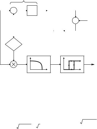
FIGURE 12.28

Block diagram of a (tuned or frequency-selective) audio tone decoder PLL.

Taking the reference phase input, θ1 = 0, the transfer function between θo and Vp can be written:

The undamped natural frequency of this PLL is ωn = aKpKf Kv r/s; its damping factor is ξ = KpKf Kv (2 a). These parameters relate to the system’s response to changes in the phase-shifting voltage, Vp, and have nothing to do with the input carrier frequency, ω1. The steady-state phase shift at lock

is simply θoss = Vp /Kp.

A third example of PLL applications examines a tone decoder, that is, a PLL system that outputs a logic HI when a sinusoidal signal is present at its input that has a frequency, f1, within some ±Δfc. Note that f1/ fc defines a capture “Q” for the tone decoder. Figure 12.28 illustrates the block diagram of a tone decoder PLL. Note that this system uses two phase detectors of

the quadrature (multiplicative) type. In the absence of a sinusoidal input signal, x1, Vc 0 and the VCO output frequency is by design ωo = b = 2π(440) r/s. Also, x6 = LO. The PLL acquires lock if the input sinusoid, x1 = A sin(ω1 t),

lies within the capture range of ±Δωc around ω1. Once the loop acquires lock, x2 = B cos(ω1 t), x3 = B sin(ω1 t), and x4 = x3 x1 = (AB/2)[cos(0) − cos(2ω1 t)].

After the LPF, x5 = AB/2 and x6 = 1 (HI). It can be shown (Grebene, 1971) that lock occurs when the input frequency ω1 lies in the capture range, given by:

© 2004 by CRC Press LLC

FIGURE 12.29

Root locus diagram for the PLL tone decoder.

where F(jΔωc) is the loop filter’s gain magnitude at ω = Δωc r/s, F(s) = (1/τ)/(s + 1/τ), and KT ∫ Kp Kv F(0). The lock range of input frequency over which the PLL will maintain lock is given by ΔωL = KT > Δωc. Thus, the tone decoder PLL behaves like a nonlinear tuned filter.

In order to design the system to respond to A440 to within ±1%, the PLL must acquire f1 = 440 ± 4.4 Hz. Thus, fc = 8.8 Hz. It is also necessary that

the loop damping factor be ξ = 0.707. The PLL’s loop gain is simply:

From AL(s), using the root-locus technique, one can find the value of the gain product KpKv to put the PLL’s closed loop poles at s* = −1/2τ ± j 2τ. (See Figure 12.29.) The RL magnitude criterion indicates:

KpKv τ = [ 2(2τ)]2

¬

© 2004 by CRC Press LLC