basic electronic design principles, and band-pass filtering. First, commonly used methods for describing stationary random noise will be examined.

9.2Descriptors of Random Noise in Biomedical Measurement Systems

9.2.1Introduction

When stationarity is assumed for a noise source, averages over time are equivalent to ensemble averages. An ensemble average is carried out at a given time on data from N separate records that are generated simultaneously from a stationary random process (SRP) (in the limit N •). If the stationary random process is ergodic, then only one record needs to be examined statistically because it is “typical” of all N records from the SRP.

An example of a nonstationary noise source is a resistor that, at time t = 0, begins to dissipate average power such that its temperature slowly rises above ambient, as does its resistance. (As demonstrated later, the meansquared noise voltage from a resistor is proportional to its Kelvin temperature.)

Probability and statistics are used to describe random phenomena. Several statistical methods for describing random noise include but are not limited to the mean; the root-mean-square (RMS) value; the probability density function; the crossand autocorrelation functions and their Fourier transforms; the crossand autopower density spectra (PDS); and the root power density spectrum (RPS, which is simply the square root of the PDS). The PDS and RPS are, in general, functions of frequency. These descriptors are treated in detail next.

9.2.2The Probability Density Function

The probability density function (PDF) is a mathematical model that describes the probability that any random sample of a noise function, n(t), will lie in a certain range of values. The univariate PDF considers only the amplitude statistics of the noise waveform, not how it varies in time. The univariate PDF of the SRV, n(t), is defined as:

where x is a specific value of n taken at some time, t, and dx is a differential increment in x. The mathematical basis for many formal derivations and proofs in probability theory, the PDF has the properties:

© 2004 by CRC Press LLC

Several PDFs are widely used as mathematical models to describe the amplitude characteristics of electrical and electronic circuit noise. These include:

In Equation 9.5, ∙x® is the true mean or expected value of the stationary random variable (SRV), x, and σx2 is the variance of the stationary random variable (SRV), x, described next. The true mean of a stationary ergodic noisy voltage can be written as a time average over all time:

The mean of the SRV, x, can also be written as an expectation or probability average of x:

© 2004 by CRC Press LLC

Similarly, the mean squared value of x can be expressed by the expectation or probability average of x2:

The mean can be estimated by a finite average over time. For discrete data, this is called the sample mean, which is a statistical estimate of the true mean and as such has noise itself.

The variance of the random noise, σx2, is defined by:

It easy to show from this equation that ∙x2® = σx2 + ∙x®2, or E{x2} = σx2 + E2{x}. Because the random noise to be considered has zero mean, the mean squared

noise is also its variance.

Under most conditions, it is assumed that the random noise arising in a biomedical measurement system has a Gaussian PDF. Many mathematical benefits follow this assumption; for example, the output of a linear system is Gaussian with variance σy2 given the input to be Gaussian with variance σx2. If Gaussian noise passes through a nonlinear system, the output PDF generally will not be Gaussian; however, this chapter will show ways of describing the transformation of Gaussian input noise by a nonlinear system.

9.2.3The Power Density Spectrum

A noise source can be thought of as the sum of a very large number of sine wave sources with different amplitudes, phases, and frequencies. Very heuristically, a power density spectrum (PDS) shows how the mean squared values of these sources is distributed in frequency.

© 2004 by CRC Press LLC

One approach to illustrate the meaning of the PDS of the noise, n(t), uses the autocorrelation function (ACF) of the noise. The ACF is defined in the following by the continuous time integral (Aseltine, 1958):

Because Rnn(τ) is an even function, its Fourier transform, Φnn(ω), is also an even function; stated mathematically, this means:

The following discussion will also consider the one-sided PDS, Sn(f ), which is related to the two-sided PDS by:

Note that the radian frequency, ω, is related to the Hertz frequency simply by ω = 2πf.

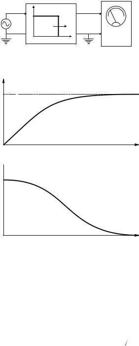
To see how to find the one-sided PDS experimentally, examine the model system shown in Figure 9.1(A). Here, a noise voltage is the input to an ideal low-pass filter with an adjustable cut-off frequency, fc. The output of the ideal low-pass filter is measured with a broadband, true RMS, AC voltmeter. Begin with fc = 0 and systematically increase fc, each time recording the square of the RMS meter reading, which is the mean squared output voltage, von2 , of the filter. As fc is increased, von2 increases monotonically, as shown in Figure 9.1(B). Because of the finite bandwidth of the noise source, von2 eventually reaches an upper limit, which is the total mean-squared noise voltage of the noise source. The plot of von2 ( fc) vs. fc is called the cumulative mean-squared noise characteristic of the noise source. In this example, its units are mean-squared volts.

© 2004 by CRC Press LLC

Sn(f)

(MSV/Hz)

f

0

0

C

FIGURE 9.1

(A) System for measuring the integral power spectrum (cumulative mean-squared noise characteristic) of a noise voltage source, eN( f ). (B) Plot of a typical integral power spectrum. (C) Plot of a typical one-sided power density spectrum. See text for description.

A simple interpretation of the one-sided noise power density spectrum, Sn(f ), is that it is the derivative, or slope, of the cumulative mean-squared noise characteristic curve described previously. Stated mathematically, this is:

© 2004 by CRC Press LLC

A plot of a typical noise PDS is shown in Figure 9.1(C). Note that a practical PDS drops off to zero as f •.

Those first encountering the PDS concept sometimes ask why it is called a power density spectrum. The power concept has its origin in the consideration of noise in communication systems and has little meaning in the context of noise in biomedical instrumentation systems. One way to rationalize the power term is to consider an ideal noise voltage source with a 1-ohm load. In this case, the average power dissipated in the resistor is simply the total mean-squared noise voltage (P = von2 /R).

From the preceding heuristic definition of the PDS, it is possible to write the total mean-squared voltage in the noise voltage source as the integral of the one-sided PDS:

The mean squared voltage in the frequency interval, (f1, f2), is found by:

Often noise is specified or described using root power density spectra, which are simply plots of the square root of Sn(f ) vs. f, and have the units of RMS volts (or other units) per root Hertz.

Special (ideal) PDSs are used to model or approximate portions of real PDSs. These include the White noise PDS and the one-over-f PDS. A white noise PDS is shown in Figure 9.2(A). Note that this PDS is flat; this implies that

which is clearly not realistic. A 1/f PDS is shown in Figure 9.2(B). The 1/f spectrum is often used to approximate the low-frequency behavior of real PDSs. Physical processes that generate 1/f-like noise include ionic surface phenomena associated with electrochemical electrodes; carbon composition resistors carrying direct current (metallic resistors are substantially free of 1/f noise); and interface imperfections affecting diffusion and recombination phenomena in semiconductor devices. The presence of 1/f noise can present problems in the electronic signal conditioning systems used for low-level, low-frequency, and dc measurements.

© 2004 by CRC Press LLC